RESEARCH ARTICLE  |
Assessment of formation brine salinity, pressure and temperature in selected structures in eastern Denmark and implications for CO2 storage
Niels H. Schovsbo*1 , Hanne D. Holmslykke2, Anders Mathiesen3, Carsten M. Nielsen1
Abstract
CO2 storage presents new risks and challenges, where the properties of formation water play an important role. These challenges include reduced injectivity and storage capacity due to salt precipitation, viscous fingering caused by viscosity contrasts between CO2 and brine and diminished CO2 solubility in formation waters. Understanding these factors and developing predictive models for pressure distribution are essential for successful CO2 storage projects. This study presents salinity (Cl and total dissolved solids), density, temperature, pressure, halite (NaCl) saturation, CO2 solubility and viscosity of formation waters across five CO2 storage sites in Denmark (Stenlille, Gassum, Rødby, Lisa and Inez), covering eight reservoirs (one in the Frederikshavn Formation, four in the Gassum Formation and three in the Bunter Sandstone and Skagerrak Formations). Salinity assessments are based on existing brine data or, where unavailable, a reference salinity model developed from a water chemistry database with 77 analyses from 28 wells in the Danish Basin and adjacent regions. The model was created using Partial Least Squares regression, accounting for local geological developments and subsurface salts. We report high chloride levels (182 000–202 000 mg/L) and densities (1.21–1.23 kg/L) in the Bunter Sandstone and Skagerrak Formations, while the Gassum and Frederikshavn Formations are undersaturated with halite, exhibiting lower chloride levels (99 000–148 000 mg/L) and densities (1.11–1.17 kg/L). These differences suggest a higher risk of mineral precipitation due to brine evaporation in dry CO2, and a higher risk of density override due to significant density contrast, which will hamper filling efficiency in older reservoirs. Modelling shows that CO2 solubility reaches 33.9 g CO2/L, with a 37% reduction due to chemical and pressure–temperature variations. Conceptual fluid flow modelling is recommended to further assess brine–rock–CO2 interactions. The salinity model has implications for geothermal reservoir assessment and can be applied regionally.
Citation: Schovsbo et al. 2025: GEUS Bulletin 60. 8383. https://doi.org/10.34194/62417j08
Copyright: GEUS Bulletin (eISSN: 2597-2154) is an open access, peer-reviewed journal published by the Geological Survey of Denmark and Greenland (GEUS). This article is distributed under a CC-BY 4.0 licence, permitting free redistribution, and reproduction for any purpose, even commercial, provided proper citation of the original work. Author(s) retain copyright.
Received: 06 Oct 2024; Revised: 17 Dec 2024; Accepted: 27 Jan 2025; Published: 21 May 2025
Competing interests and funding: No competing interests declared.
This study is funded from the GEUS CCS2020–2024 project for maturation of selected structures to CO2 storage site.
*Correspondence: nsc@geus.dk
Keywords: brine–CO2 dynamics, CO2 solubility, fluid–rock interaction, geochemical modelling, halite saturation, viscous fingering
Abbreviations:
GEUS: Geological Survey of Denmark and Greenland
PLS: Partial Least Squares
Pw: hydrostatic pressure
scCO2: Supercritical CO2
SI: Saturation Index
SRM: Spatial Relationship Matrix
T: Temperature
TDS: Total dissolved solids
δw: brine density
μ: viscosity
Edited by: Jon Ineson (GEUS, Denmark)
Reviewed by: Philip Ringrose (NTNU, Norway), Kim H. Esbensen (KHE Consulting, Denmark)
1. Introduction
Deep underground storage of CO2 in suitable saline aquifers or depleted oil and gas reservoirs represents a significant strategy to mitigate global warming caused by high levels of anthropogenic CO2 emissions (IPCC 2023). In Denmark, there are many porous rock formations, which offer a high technical CO2 storage potential, with multiple large structures suitable for storage of dense, supercritical (sc)CO2 (Hjelm et al. 2022; Gregersen et al. 2025, this volume). Over recent years, characterising these sites to advance their development into CO2 storage facilities has been a major focus for the Geological Survey of Denmark and Greenland (GEUS; Hjelm et al. 2022; Gregersen et al. 2023, 2025; Abramowitz et al. 2024; Bjerager et al. 2024; Fyhn et al. 2024; Keiding et al. 2024).
The primary reservoirs under investigation onshore Denmark and in the eastern part of the offshore sector (Fig. 1) are Triassic to Jurassic sandstones (Bunter Sandstone, Skagerrak and Gassum Formations, Fig. 2) that form regional aquifers. The presence of high salinity formation water in these aquifers has been well-documented since the 1940s, marking the beginning of hydrocarbon exploration activities. An initial survey of formation water chemistry was conducted by Dinesen (1961), which was further elaborated by Laier (1989a, 1989b, 2002, 2008). Traditionally, the discussion around formation water chemistry has been focused on implications for geothermal energy production, particularly concerning the risks associated with steel corrosion in highly saline environments and the potential for scale and mineral precipitation, which can severely impact operational efficiency and safety (Laier 2002; Holmslykke et al. 2019, 2023; Kazmierczak et al. 2022).

Fig. 1 Location of wells and potential CO2 storage sites (structures) mentioned in the text. Well name abbreviations: ER-4S: Erslev-4S. Fa-1: Farsø-1. Ga-1: Gassum-1. Ha-1: Haldager-1. Hö-2: Höllviken-2. Hö-1: Höllviksnäs-1. In-1: Inez-1. FCC-1: Malmö/FCC-1. Ma-1: Margretheholm-1. Ma-2: Margretheholm-2. Rø-1: Rødby-1. St-1–6: Stenlille-1, Stenlille-2, Stenlille-3 Stenlille-4 Stenlille-5 and Stenlille-6. St-19: Stenlille-19. Stv-1: Stevns-1. Sø-1A: Sønderborg-1A. Sø-2: Sønderborg-2. Th-2: Thisted-2. Th-3: Thisted-3. Tø-1: Tønder-1. Tø-4: Tønder-4. Tø-5: Tønder-5. Ør-1: Ørslev-1. Aa-1A: Aars-1A. Aar-02: Aarhus-02.

Fig. 2 Mesozoic stratigraphy of the studied area. Reproduced from Gregersen et al. (2025, this volume).
With the resurgence of interest in the Triassic and Jurassic reservoirs for CO2 storage applications, the need for pre-drilling assessments of formation water characteristics for specific structures, along with regional mapping of water properties such as density, has gained prominence. Moreover, CO2 storage introduces novel risks and challenges where formation water plays a key role. These include the risk of injection and storage capacity reduction due to salt precipitation as a result of reservoir dry-out (Pruess 2009; Ringrose 2020; Edem et al. 2022; Cui et al. 2023; Worden 2024) and complications from viscous fingering arising from significant density and viscosity contrasts between brine and scCO2, which may impede the effective distribution of CO2 throughout the reservoir (Kumar et al. 2020; Ringrose 2020). Additionally, the solubility of CO2 in formation water decreases as salinity increases, which can significantly diminish CO2 dissolution and, consequently, the overall efficiency of CO2 sequestration (Holloway 2005; Deng et al. 2018). In addition, maintaining pressure control in the reservoir by discharging formation water may be a key component for maintaining caprock and reservoir integrity (Dewar et al. 2022). However, the environmental impact arising from such discharge must be assessed, including the possible mixing ratio with seawater, as even a slight increase in salinity compared to ambient levels is regarded as harmful to the aquatic environment. Understanding these interactions and developing accurate predictive models are essential for the design and successful implementation of CO2 storage projects.
In this study, we use existing databases to conduct assessments of various Mesozoic structures that formed part of the GEUS-led Carbon Capture and Storage study, CCS2022–2024, focused on maturing potential CO2 storage sites (Gregersen et al. 2023, 2025; Fig. 1). The objective is to assess the key physical properties of the formation water including its temperature, pressure, salinity (Cl and total dissolved solids (TDS)) and density, to discuss the effects hereof on the CO2 storage efficiency and hence to highlight injection risks. In order to evaluate salinities in structures and reservoir levels where no water analyses are available, we have developed a methodology based on the well-documented depth dependencies identified in previous research (Laier 1989a, 2008; Holmslykke et al. 2019) that aims to refine our predictions by aligning them more closely with the specifics of the local geology using the methodology presented in Schovsbo et al. (2020). We use the term ‘reservoir’ here as an informal zone of a lithostratigraphical unit to describe a porous unit suitable for CO2 storage.
2. Geological setting
Gregersen et al. (2025, this volume) have recently described the geological development including basin tectonics and history of the Danish Basin and North German Basin and the reader is referred to this publication for a detailed account. Here, we provide a more focused description highlighting the geological and deposition characteristics that are most relevant for the evaluation of formation water salinity.
The structural configurations of the Danish Basin and the North German Basin (Fig. 1) were established during the early Permian (Michelsen et al. 2003). In the central part of the Danish Basin, the post mid-Permian succession attains thicknesses up to 9000 m (Fig. 3D). The upper Permian succession (Zechstein Group) is characterised by extensive evaporite deposits, particularly in the major depocentres, with carbonate upon and fringing paleo highs (Ziegler 1990; Geluk 2000; Fig. 3A). Evaporite accumulation waned in the earliest Triassic, when sedimentation of non-marine siliciclastics dominated the area, but resumed in the late Early Triassic. In the North German Basin, evaporites accumulated during the extensional tectonics of the Hardegsen phase, forming the Röt Basin in the latest Early Triassic (Kovalevych et al. 2002; Fig. 3B). In Denmark, correlative deposits are represented by the Ørslev Formation (Fig. 2), an evaporitic claystone unit that includes rock salt (mostly halite) deposits in the deeper parts of the basin (Bertelsen 1980). The northern limit of the halite facies in the Ørslev Formation towards the Ringkøbing–Fyn High is somewhat uncertain but has been re-evaluated based on well logs and cuttings during the preparation of the Geothermal WebGIS Portal and likely extend north up to the Ringkøbing Fyn High (see Vosgerau et al. 2016; Fig. 3B).

Fig. 3 Maps showing extension of rock salt in (A) the Zechstein, (B) the Röt (Ørslev Formation), and (C) the Oddesund Formation and (D) the depth to the Pre Zechstein surface. A is modified after Geluk (2000), B after Kovalevych et al. (2002) and Vosgerau et al. 2016 (WebGIS Röt salt risk map that highlights a high-risk area for rock salt presence), C after Bertelsen (1980) and D after Vejbæk & Britze (1994).
Evaporite accumulation resumed in the Late Triassic. Although the Upper Triassic in the Danish Basin and the North German Basin is predominately characterised by terrestrial siliciclastics, evaporitic conditions prevailed locally in the former basin during deposition of the Oddesund Formation (Bertelsen 1980). This is typically an evaporite-bearing claystone succession, but significant rock salt deposits have been detected in central depocentres of the Danish Basin (Fig. 3C). Additional mapping associated with the CCS2022–2024 project has shown that Oddesund evaporites are not limited to these areas but may have formed in paleo lows elsewhere in the basin (Fyhn et al. 2024).
In the context of CO2 storage potential, the key Mesozoic reservoirs in the Danish subsurface are the braided river and aeolian sandstones of the Lower to Mid Triassic Bunter Sandstone and Skagerrak Formations, deposited under arid to semi-arid conditions, and the Upper Triassic – Lower Jurassic Gassum and the Cretaceous Frederikshavn Formations, deposited in paralic and shallow marine environments (Fig. 2). The Bunter Sandstone Formation is the main Triassic reservoir unit in the North German Basin and the Danish Basin, reaching thicknesses of up to 300 m (Bertelsen 1980); within the Danish Basin, this formation grades laterally into the temporally equivalent lower levels of the Skagerrak Formation at the basin margin (Bertelsen 1980; Nielsen 2003; Weibel & Friis 2004; Gregersen et al. 2025; Keiding et al. 2024).
The Gassum Formation represents the main reservoir sandstone unit in the area; it exhibits thicknesses ranging from 50 to 150 m across both the North German Basin and the Norwegian–Danish Basin, though it is absent over the Ringkøbing–Fyn High and thins into the Fennoscandian Border Zone. Marine conditions were established from the Late Triassic through the Early Jurassic, the transgressive development being recorded by the restricted marine Vinding Formation, the fluvial to shallow marine Gassum Formation and the offshore marine Fjerritslev Formation (Fig. 2). Mid-Jurassic uplift led to the erosion and truncation of the Fjerritslev Formation. Subsequent marine deposition included the accumulation of additional secondary sand-rich reservoirs such as the Middle Jurassic Haldager Sand Formation and the Lower Cretaceous Frederikshavn Formation.
3. Data and methods
3.1. Geochemical database
We use the geochemical database of formation water compositions originally compiled by Laier (1989a, 2008), now augmented with new data from Holmslykke et al. (2019) covering the Sønderborg, Thisted and Margretheholm geothermal test sites. Additional contributions include data from Laier (1989b) from the Stenlille area, from Bonnesen et al. (2009) concerning the deepest section of the Stevns-1 research well (at 450 m) to limit the contributions of meteoric water in the shallower parts (Bonnesen et al. 2009) and a Zechstein Group water sample from the Ørslev-1 well (Gulf Denmark 1968, p. 36). Data also comes from the geothermal well DGE-1 that tested the basement in Scania (Rosberg & Erlström 2022) and from the geothermal well Aarhus-02 that tested the Gassum Formation between 2293 and 2411 m (Fig. 1). We excluded data from the topmost section (above 200 m) of the shallow Erslev-4S well due to the high likelihood of groundwater contamination (Laier 1989a; Bonnesen et al. 2009). The database now encompasses 28 wells (Fig. 1) and 77 brine analyses (detailed in Supplementary Table S1).
As noted by Laier (1989a, 2008), data on formation water composition are derived from two principal sources: well tests conducted during exploration or production tests conducted at geothermal plants or natural gas storage sites. The first source often presents significant uncertainties regarding contamination from the drilling process, in contrast to the latter, which offers more reliable data but with considerably more limited geographical coverage. Consistent with approaches in previous data compilations, our study incorporates both types of data, including brine extracted from core samples (Supplementary Table S1).
Our analytical data span more than 75 years of laboratory and methodological development, introducing a layer of uncertainty to our analysis. However, we have focused on the main conservative element, notably chloride (Cl), which mitigates some of the potential issues related to data variability over time. The charge balance of the water analysis containing all major ions was calculated using the software programme PHREEQCv3 (Parkhurst & Appelo 2013). The results indicate charge balance errors less than ±3% with a few samples with a charge balance error of up to –5.6% (Supplementary Table S1). Charge balances of up to 5% are typically deemed acceptable for diluted samples (Appelo & Postma 2005). Thus, the data on the formation water composition were presumed robust considering the high salinity of the samples.
3.2. Methods
3.2.1. Estimation of total dissolved solids
The total dissolved ions in a sample represent the sum of all analysed ions. For samples without a full composition analysis, we use an empirical relationship between chloride and TDS. The relationship is established from the Mesozoic reservoirs in Fig. 4 and is given by:

Fig. 4 Empirical relationships between chloride and TDS concentrations established for Mesozoic reservoirs. Based on data in Laier (2008) and Holmslykke et al. (2019).

In Eq. (1), the empirically determined coefficient 1.656 is slightly higher than that expected for a pure NaCl solution (1.649), indicating that while NaCl is the predominant ion pair, other ions such as Ca and K are also present (see also Holmslykke et al. 2019).
3.2.2. Brine density, halite saturation and CO2 solubility
Using the computer software programme PHREEQCv3 (Parkhurst & Appelo 2013) and its Pitzer database, we calculated the brine density (δw) and halite (NaCl) Saturation Index (SINaCl) at both ambient and reservoir conditions (i.e. at in situ pressure and temperature), the CO2 solubility at reservoir conditions using the Peng–Robinson equation of state and the density of fully CO2-saturated formation water (δwCO2) at reservoir conditions. Due to the interactions of different ions, this could only be performed for samples with a full composition analysis (Table 2 and 3).
For samples with measured chloride concentrations but with no full compositional analysis, we used Eq. (1) to calculate TDS and then ambient δw from Collins (1987) using Eq. (2):

Comparison between δw calculated from a full composition analysis using PHREEQC with δw calculated using Eq. (2) shows similar results with a deviation of only 0.01 kg/L between the two estimates.
The halite saturation state of the brines is indicated by the SINaCl whereby positive and negative values indicate super-saturation and undersaturation, respectively. Formation water with a SINaCl value within the range –0.4 ≤ SINaCl ≤ +0.4 is assumed to be saturated, and thus in equilibrium with halite. The range accounts for the uncertainties associated with the difficulties of sampling brines at high temperature and pressure, the analytical uncertainty and the application of thermodynamic equilibrium constants on mineral phases in saline systems (Holmslykke et al. 2019). The SINaCl value could only be calculated for samples in which both Na and Cl were measured.
3.2.3. Hydrostatic pressure and temperature
The Danish Basin and the Danish part of the German Basin are considered normally pressured based on experience gained from drilling activities, and the hydrostatic pressure (Pw) is calculated using GEUS’ own regional pressure model:

where 0.1054 bar/m is the regional pressure gradient. The gradient is often assumed to be invariant, but in practice, the gradient depends on the brine salinity, which is known to be a function of depth (Laier 1989a). Hence the gradient in Eq. (3) should be viewed as an average of the changing brine densities in the Gassum Formation. Validation of the pressure model with in situ measurements could only be made for the Stenlille area (Fig. 1) where the predicted Pw in the Gassum Formation using Eq. 3 and measured Pw in the Stenlille-5 well is within 4 bar. For the more saline and hence more dense brine in the Bunter Sandstone and Skagerrak Formations, the estimated hydrostatic pressures should be regarded as minimum pressure estimates.
Formation temperatures are calculated from Fuchs et al. (2019). For the Stenlille area, we assume that the temperature model for Stenlille-1 (Fuchs et al. 2019) applies to all Stenlille wells. For Gassum-1 and Rødby-1, where no thermal gradients were reported by Fuchs et al. (2019), we use:

where the thermal gradient is 27°C/km and the surface temperature is 8°C as used in the deep geothermal evaluation of Denmark (Vosgerau et al. 2016).
3.2.4. Brine viscosity
Brine (NaCl) viscosity (μbrine), is calculated as a function of temperature and NaCl concentration according to the correlation developed by Phillips et al. (1981):

where a = 0.0816, b = 0.0122, c = 0.000128, d = 0.000629, k = –0.7, T = Temperature (°C), M = molal concentration (mol NaCl/kg H2O), μw = viscosity of water (cP). The concentration of NaCl is calculated from the TDS content assuming a pure NaCl solution. μw is estimated from table provided by the National Institute of Standards and Technology by the U.S. Department of Commence (Linstrom & Mallard 2023). Francke & Thorade (2010) compared the relationship given in Eq. (5) to models by Kestin et al. (1981) and Mao & Duan (2009) and demonstrated consistent values and a deviation below 0.9%.
3.2.5. CO2 density and viscosity
CO2 density (δCO2) and viscosity (μCO2) at reservoir conditions are estimated from tables provided by the NIST Chemistry Webbook.
3.2.6. Partial least squares regression analysis
The Partial Least Squares (PLS) multivariate regression method was employed to explore relationships between chloride concentrations and depth, in relation to the main stratigraphic tops and facies. The multivariate X data were prepared from depths in relation to the listed stratigraphic tops in Table 1. Thus, the depth of a brine sample was calculated relative to any given datum by determining its depth above (positive value) or below (negative value) the datum, resulting in a matrix termed as the Spatial Relationship Matrix (SRM; Fig. 5). This approach facilitates the development of predictive models (see Schovsbo et al. 2020). The PLS regression enables direct modelling of correlations between the dependent Cl variable (y) and the multivariate independent depth variables (X), based on the collinearity among X variables (Esbensen & Swarbrick 2018). The PLS regression model was cross-validated by randomly splitting the data into two segments – an independent training set and a test data set – ensuring a realistic prediction performance validation (Esbensen & Geladi 2010; Esbensen & Swarbrick 2018). All data were auto-scaled, and the modelling was performed in the software package Unscrambler® 10.5 by CAMO (Esbensen & Swarbrick 2018).

Fig. 5 Principle of the Spatial Relationship Matrix (SRM). The transformation expresses the sample depth relative to a specific surface by calculating its depth above (positive value) or below (negative value) the datum. Consequently, a sample in a well with ‘n’ identified surfaces will have n depths. S1: Surface 1. S2: Surface 2. S3: Surface 3. S4: Surface 4.
4. Results
4.1. Salinity prediction
Laier (2008) discussed methods for predicting water composition in reservoirs lacking direct analyses. One approach, originally presented by Laier (1989a), involves using a simple model that correlates chloride concentration with present-day depth by plotting Cl concentrations versus depth. Figure 6A presents a similar depth plot for the full augmented database (Supplementary Table S1). The overall relationship has an r² of 0.65, reflecting that only 65% of the total data variance can be modelled by a simple correlation relationship (Fig. 6A).

Fig. 6 Chloride concentrations versus present day depth below ground level (A) and Brine-halite (NaCl) Saturation Index (SINaCl) at reservoir conditions (B). Thermodynamic equilibrium for halite (–0.4 ≤ SINaCl ≤ 0.4) is illustrated with a grey band. Well abbreviations as Fig. 1. Broken lines in A indicate sub-trends discussed in the text. The DGE-1 well tested crystalline basement between 3198 and 3702 m of depth. Aarhus-02 (Aar-02) tested the interval 2293–2411 m.
As discussed by Laier (1989a), the depth relationship in Fig. 6A encompasses several sub-trends:
- The Tønder samples, representing partly halite-cemented Bunter Sandstone (Laier & Nielsen 1989; Hjuler et al. 2019), plot with high and apparently invariant Cl–depth relationships.
- The Erslev-4S data exhibit a steep Cl–depth gradient, reflecting the intrusion of shallow salt diapirs into the ground water zone.
- The bulk of the Gassum and younger reservoirs plot with a relatively well-defined Cl–depth relationship.
Laier (1989a) also noted the wide range of chloride levels in the Skagerrak samples, from 110 000 ppm at Margretheholm (2550 m depth) to 200 000 ppm at Stenlille-19, despite both being at nearly the same depth. These variations render the depth plot alone less effective for predicting chloride concentrations in unsampled reservoirs. Consequently, Laier (2008) proposed an alternative approach that combines analogue considerations between reservoirs of known and unknown compositions, applying adjustments for depth differences based on Laier (1989a). Using this method, the likely brine compositions for seven reservoirs at specific locations and depths were determined.
4.2. Partial least squares regression model of salinity
4.2.1. Modelling concepts
To develop a mathematical model for the relationship between chloride concentrations and depth, we began by identifying the fundamental controls influencing salinity in formation brines.
To determine if the variation is controlled by saturation-induced constraints, we calculated the saturation state of the formation water with respect to halite (brine–halite SI) under reservoir conditions. We then plotted this against the depth below ground level for water samples with a full compositional analysis (Fig. 6B). The analysis indicates that, except for the very deep (>2.5 km) reservoirs in Aars-1A and Farsø-1, all samples from the Gassum and younger reservoirs are undersaturated with respect to halite. In contrast, all water samples from the Bunter Sandstone, Skagerrak, Ørslev and Falster Formations (except those from Margretheholm), and from the Zechstein Group, are in equilibrium with halite (Fig. 6B).
To determine the geographical component, we observed that the salinity variation in the Bunter Sandstone and Skagerrak Formations differs between the North German Basin, the Danish Basin and the Øresund Basin that forms a marginal part of the Danish Basin. Within these basins, the Tønder area in the North German Basin has highest salinities, and the Margretheholm and Höllviksnäs areas in the Øresund Basin are the least saline (Fig. 6A). The subsurface rock salt occurrence presented in Fig. 3A, B, C was compared with sample locations for water chemistry (Fig. 7). We observed that, for the Bunter Sandstone and Skagerrak Formations, the primary control on salinity levels appears to be stratigraphic proximity to rock salt in the Zechstein Group and the Ørslev and Oddesund Formations as rock salt is present in the North German Basin and Danish Basin but absent in the Øresund Basin.

Fig. 7 Assignment of the categorial contribution variables for North German Basin (CNGB) and Danish Basin (CDB) for the PLS regression analysis of Zechstein, Bunter Sandstone, Ørslev, Falster and Skagerrak brine samples. A value of 1 indicates the likely presence of interbedded rock salt and a value of 0 indicates the likely absence. Assessed potential CO2 structures (yellow) and wells are after Fig. 1.
To account for this, we incorporated information on the presence or absence of rock salt into the PLS regression model reflecting the proximity to, or absence of, interbedded rock salt layers within each basin. This was accomplished by introducing parameters labelled CNGB and CDG in Fig. 7, representing categorical contribution variables from the North German Basin and the Danish Basin, respectively. To model the depth trend in the chloride concentrations, we employed an analysis of the stratigraphical data from the wells by calculating the depth of the brine samples to the given stratigraphical surfaces resulting in a SRM of the brine sample depths. This approach follows that of Schovsbo et al. (2020), who modelled depth trends in vitrinite reflectance data from North Sea wells by incorporating stratigraphical data. The SRM (see Fig. 5) enables stratigraphical data to be modelled using multivariate statistical tools, such as PLS regression.
4.2.2. Partial least squares model results
For preparation of the SRM, stratigraphical information was obtained for Danish wells from Nielsen & Japsen (1991) with updates from Gregersen et al. (2023), Abramowitz et al. (2024), Keiding et al. (2024) and for Swedish wells from Erlström & Sivhed (2012) and Erlström et al. (2018). The Eg(S)-1 well, the shallow research well Stevns-1 that only penetrated the upper part of the Chalk Group (Stemmerik et al. 2006) and the Haldager-1 well that terminated in the Fjerritslev Formation were not included due to limited stratigraphical coverage. In addition, the DGE-1 well that tested the crystalline basement between 3198 and 3702 m in Scania was excluded due to uncertainties concerning the depths of the water analyses.
In the SRM, we used the sample depth calculated in relation to the following surfaces: ground level, top Chalk Group, top Lower Cretaceous, top Upper Jurassic, top Middle Jurassic, top Triassic (equivalent to the top Gassum Formation) and the top middle Triassic (equivalent to top Vinding Formation or base Gassum Formation). To account for the chloride contribution from interbedded rock salt in the Zechstein Group and the Ørslev and Oddesund Formations to the Bunter Sandstone, Falster and Skagerrak reservoirs, categorical contribution variables, CNGB and CDB were assigned according to Fig. 7. A CNGB value of 1 indicates the presence of the well within the depositional areas of the Zechstein Group and the Ørslev Formation in the North German Basin, while a CDB value of 1 signifies the presence of the well within the depositional area of rock salt from the Zechstein Group and/or the Oddesund Formation in the Danish Basin (Fig. 7). Wells outside these areas, such as Margretheholm-1 and -2 and Swedish wells in the Øresund Basin (Erlström et al. 2018), were assigned a CDB value of 0. For Gassum and younger reservoirs, both CNGB and CDB are assigned a value of 0.
The resulting PLS regression model of the chloride concentrations is presented in Fig. 8. The full input variable [SRM, CNGB, CDB] data are available in Supplementary Table S2. The proportions of total data variance modelled shown along each PLS component [X%, Y%] are shown in Fig. 8B. From this diagram, a three-component PLS model on the [SRM, CNGB, CDB] variable set predicts chloride levels with very satisfactory validation results, as seen in the prediction versus reference plot in Fig. 8C (slope 0.95; r2 = 0.95). Hence, the PLS regression model exhibits a correlation between measured chloride levels and predicted chloride levels that is much stronger than could be established from using only the depth below surface for predicting the chloride concentrations (r2 = 0.65; Fig. 6A).
![Fig. 8 PLS-regression model for chloride concentrations (red) and stratigraphic and geologic parameters [SRM, CNGB, CDB] variable set (black dots). (A) loading-weights plot (w1–w2); proportions of total data variance modelled shown along each PLS component [X%, Y%]. (B) modelled y-variance and (C) prediction versus reference plot. Proportions of total data variance (PLS factor 3) modelled shown along each PLS component [X%, Y%]. Categorial contribution variables for North German Basin (CNGB) and Danish Basin (CDB). CL: chloride. Other abbreviations after Table 1.](https://geusbulletin.org/index.php/geusb/article/download/8383/version/2880/14569/51637/8383_F0008_Large.jpg "Click to Enlarge View")
Fig. 8 PLS-regression model for chloride concentrations (red) and stratigraphic and geologic parameters [SRM, CNGB, CDB] variable set (black dots). (A) loading-weights plot (w1–w2); proportions of total data variance modelled shown along each PLS component [X%, Y%]. (B) modelled y-variance and (C) prediction versus reference plot. Proportions of total data variance (PLS factor 3) modelled shown along each PLS component [X%, Y%]. Categorial contribution variables for North German Basin (CNGB) and Danish Basin (CDB). CL: chloride. Other abbreviations after Table 1.
The resulting PLS regression model is described by:
Gassum and younger reservoirs:

where b is a well-specific constant calculated from:
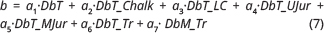
using coefficients for a1–a7 for the stratigraphical depths calculated in the well as presented in Table 1. Values for b for the analysed wells are presented in Supplementary Table S3.
For the Bunter Sandstone, Falster, Ørslev and Skagerrak reservoirs, an additional salinity component is calculated in addition to the chloride calculated from Eq. (6).
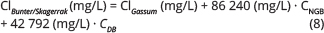
where CNGB and CDB are assigned according to Fig. 7. A reference salinity calculator based on Eqs (6), (7) and (8) is included in the Supplementary Files.
4.3. Assessment of selected reservoirs in CO2 structures
Further in the text we have evaluated the salinity (Cl and TDS), T, Pw, δw, δCO2, μCO2, μbrine, halite saturation state and the CO2 solubility in brine for selected reservoirs in five structures that are identified as suitable for CO2 storage (Gregersen et al. 2023, 2025, this volume; Abramowitz et al. 2024; Keiding et al. 2024). In our selection, we focused on drilled structures to establish stratigraphical control for the modelling. However, this is not a technical hindrance, as a pseudo well could also have been used for the assessment (see Bjerager et al. 2024 for an example). The depth profiles of the assessed chloride levels are depicted in Fig. 9 and all evaluated parameters are presented in Tables 2 and 3.
| Structure / Well | Formation | Depth (TVDGS) | Cl | TDS | Cl PLS | TDS PLS | Pw | T | CO2 solubility | SINaCl |
| m | mg/L | mg/L | mg/L | mg/L | bar | oC | g CO2/L | |||
| St-1 | Fjerritslev | 1366 | 103 000 | 169 523 | 144 | 50 | 35.1 | –0.81 | ||
| Stenlille structure | Gassum | 1506 | 106 081 | 175 670 | 159 | 54 | ||||
| St-1 | Gassum | 1506 | 108 000 | 177 894 | 159 | 54 | 33.9 | –0.76 | ||
| St-19 | Falster | 2053 | 182 000 | 302 969 | 216 | 71 | 23.1 | 0.18 | ||
| Stenlille structure | Bunter Sandstone | 2413 | 181 249 | 300 148 | 254 | 82 | ||||
| St-19 | Bunter Sandstone | 2413 | 197 000 | 322 452 | 254 | 82 | 21.5 | 0.23 | ||
| Gassum structure | Frederikshavn | 1095 | 99 437 | 164 667 | 115 | 38 | ||||
| Gassum structure | Gassum | 1545 | 115 206 | 190 782 | 163 | 50 | ||||
| Ga-1 | Ørslev | c. 2625* | 180 770 | 287 986 | 277 | 79 | 24.4 | –0.03 | ||
| Gassum structure | Skagerrak | 2795 | 201 803 | 334 185 | 295 | 83 | ||||
| Rødby structure | Bunter Sandstone | 1246 | 186 265 | 308 454 | 131 | 42 | ||||
| Inez structure | Gassum | 1650 | 107 416 | 177 881 | 179 | 50 | ||||
| Lisa structure | Gassum | 1669 | 147 772 | 244 710 | 180 | 47 | ||||
| *Depth uncertain. TVDGS: Total vertical depth below ground level / sea floor. TDS: Total Dissolved Solids. Cl PLS: Chloride concentration estimated by the PLS regression model. PW: Hydrostatic pressure at reservoir depth. T: Temperature at reservoir depth. CO2 solubility: CO2 in brine at reservoir conditions. SINaCl: Saturation state of brine–halite at reservoir conditions. | ||||||||||
| Structure / Well | Formation | Depth (TVDGS) | δw surface | δw | δCO2 | δw – δCO2 | δwCO2 | μCO2 | μbrine | μbrine / μCO2 |
| m | kg/L | kg/L | kg/L | kg/L | kg/L | cP | cP | |||
| St-1 | Fjerritslev | 1366 | 1.12 | 1.10 | 1.11 | |||||
| Stenlille structure | Gassum | 1506 | 1.12 | 0.69 | 0.43 | 0.055 | 0.71 | 12.8 | ||
| St-1 | Gassum | 1506 | 1.12 | 1.11 | 1.11 | |||||
| St-19 | Falster | 2053 | 1.21 | 1.18 | 1.18 | |||||
| Stenlille structure | Bunter Sandstone | 2413 | 1.21 | 0.68 | 0.53 | 0.056 | 0.63 | 11.2 | ||
| St-19 | Bunter Sandstone | 2413 | 1.22 | 1.20 | 1.20 | |||||
| Gassum structure | Frederikshavn | 1095 | 1.11 | 0.73 | 0.39 | 0.060 | 0.91 | 15.2 | ||
| Gassum structure | Gassum | 1545 | 1.13 | 0.73 | 0.40 | 0.061 | 0.80 | 13.0 | ||
| Ga-1 | Ørslev | c. 2625* | 1.20 | 1.18 | 1.18 | |||||
| Gassum structure | Skagerrak | 2795 | 1.23 | 0.73 | 0.50 | 0.062 | 0.66 | 10.6 | ||
| Rødby structure | Bunter Sandstone | 1246 | 1.21 | 0.73 | 0.49 | 0.060 | 1.14 | 19.0 | ||
| Inez structure | Gassum | 1650 | 1.12 | 0.75 | 0.37 | 0.064 | 0.76 | 11.8 | ||
| Lisa structure | Gassum | 1669 | 1.17 | 0.78 | 0.39 | 0.068 | 0.89 | 13.1 | ||
| *Depth uncertain. TVDGS: Total vertical depth below ground level / sea floor. δw Surface: Density of formation water at ambient conditions. δw: Density of formation water at reservoir conditions. δCO2: Density of scCO2 at reservoir conditions. δw – δCO2: Density difference between formation water and scCO2. δwCO2: Density of CO2 saturated formation water at reservoir conditions. μCO2: Viscosity of scCO2 at reservoir conditions. μbrine: Viscosity of brine (NaCl) at reservoir conditions. | ||||||||||

Fig. 9 Measured chloride concentrations and PLS-modelled chloride concentrations for measurements and reservoir levels in structures versus depth below ground level. Field of brine–halite equilibrium (grey) is based on PHREEQC simulations (Fig. 6B). For well abbreviations, see Fig. 1.
4.3.1. The Stenlille structure
The Stenlille structure is situated in the central part of the island of Sjælland in the Danish Basin (Fig. 1). The structure is a four-way closure developed on top of a Zechstein salt pillow and is currently both an active natural gas storage site and a potential CO2 storage site, with the Gassum and Bunter Sandstone Formations identified as injection possibilities (Gregersen et al. 2023). Twenty brine analyses are available from seven wells (Fig. 1, Supplementary Table S1). We use the reservoir depths from the Stenlille-1 and Stenlille-19 wells, and the full composition analysis from these wells for the Fjerritslev, Gassum, Falster and Bunter Sandstone Formations as references (Table 2).
At Stenlille, the PLS-predicted chloride concentration for the Gassum Formation matches the available composition within uncertainty (PLS 106 000 vs. measured 108 000 mg/L). However, for the Bunter Sandstone Formation at 2413 m, the PLS-estimated Cl content is 16 000 ppm too low (181 000 vs. 197 000 mg/L; Table 2). Brine density at surface conditions estimated using Eq. (4) is up to 0.03 kg/L lower than that estimated with PHREEQC based on the measured brine composition at reservoir conditions (Table 3).
The shallowest water samples at Stenlille, measured in the Fjerritslev and Gassum Formations, are undersaturated with respect to halite with SINaCl of –0.81 to –0.76, whereas the deeper water samples measured in the Falster and Bunter Sandstone Formations are in equilibrium with respect to halite (SI = 0.18 to 0.23). Due to increasing salinity with depth, CO2 solubility also decreases with depth. Thus, CO2 solubility decreases from approximately 34 g CO2/L in the Gassum Formation at 1506 m to 21.5 g CO2/L in the Bunter Sandstone Formation at 2413 m (Table 2). Supercritical CO2 will have a density of about 0.68 kg/L in both the Gassum and Bunter Sandstone Formations. Due to the higher TDS in the latter formation, the water density here is highest, resulting in a relative density difference between the two phases of 0.43 kg/L in the Gassum Formation and 0.53 kg/L in the Bunter Sandstone Formation. The viscosity (μbrine) is in the range 0.63–0.71 centipoise (cP), and the mobility ratio, calculated as the ratio between brine and CO2 viscosities, ranges from 11.2 to 12.8 with the lowest ratio in the Bunter Sandstone Formation due to its high temperature (Table 3). The relatively high mobility ratios may increase the risks of viscous fingering. The relative increase in formation water density at a CO2-saturated state (δWCO2) is 0.3% for the Gassum Formation and negligible for the Bunter Sandstone Formation (Table 3).
4.3.2. The Gassum structure
The Gassum structure is situated in central Jylland within the Danish Basin and is a four-way closure atop a Zechstein salt pillow (Fig. 1). The structure was drilled by the Gassum-1 well and is targeted for CO2 storage, with the Frederikshavn, Gassum (primary) and Skagerrak Formations as possible reservoirs (Keiding et al. 2024).
In the Gassum-1 well, a brine sample was retrieved during drilling due to uncontrolled well flow, as reported in the Final Well Report (Danish American Prospecting 1951, p. 324). Due to the conditions under which the sample was collected, the exact depth remains uncertain but is believed to represent ‘sands logged at and below 8816 feet (2687 m)’. Laier (2008) included this sample in his compilation, assigning it a depth of 2625 m and to the Falster/Skagerrak Formation. We have retained this estimate while noting that the actual depth could be somewhat deeper and consider it to represent an Ørslev Formation brine following Keiding et al. (2024; Tables 2 and 3).
Applying the PLS regression model with the Gassum-1 stratigraphy as input, it is estimated that at the depth of the Frederikshavn Formation, situated at approximately 1095 m, the brine has a chloride concentration of 99 400 mg/L (equivalent to 164 700 mg/L TDS). Within the primary reservoir of the Gassum Formation, located at roughly 1550 m below ground level, the estimated salinity reaches approximately 115 200 mg/L Cl (190 700 mg/L TDS). Meanwhile, at the depth of the Skagerrak sandstone reservoir, around 2800 m, salinity is estimated to be approximately 201 800 mg/L Cl (334 100 mg/L TDS) with a density of 1.23 kg/L. The influx at 2625 m in the Ørslev Formation is modelled to have a Cl level of 195 000 mg/L, which is 15 000 mg/L higher than measured values of 180 770 mg/L Cl, 287 986 mg/L TDS. Given the uncertainties with the depth of the influx and modelling, this seems reasonable.
Halite saturations and CO2 solubility cannot be modelled for the three reservoir levels. From Fig. 9, we assume that the brine compositions are undersaturated with respect to halite in the Frederikshavn and Gassum Formations and in equilibrium with respect to halite in the Skagerrak Formation. The influx at 2625 m in the Ørslev Formation is modelled to be in equilibrium with halite and to have a CO2 solubility of 24 g CO2/L. At this level, the increase in δW upon saturation with CO2 is negligible (Table 3). Values of δCO2 in all reservoirs are around 0.73 kg/L, which means that the density contrast between CO2 and brine is highest (0.50 kg/L) in the Skagerrak Formation and lowest in the Frederikshavn Formation (0.40 kg/L). The μbrine ranges from 0.66 to 0.91 cP and the mobility ratio (μbrine/μCO2) ranges between 10.6 and 15.2 with the lowest value in the Skagerrak Formation.
4.3.3. The Rødby structure
The Rødby structure is situated in the western part of the island of Falster in the North German Basin (Fig. 1). This structure is a four-way closure developed on a Zechstein salt pillow and is targeted for CO2 storage within the Bunter Sandstone Formation, as the Gassum Formation is too shallow to be suitable for CO2 storage (Abramowitz et al. 2024). We use the Rødby-1 well data as the basis for our analysis (Table 2) and since no brine composition analyses are available, we have used the salinity (Cl and TDS) modelled from the PLS regression model (Eq. 6) as the basis for the formation water composition.
Accordingly, we estimate the Bunter Sandstone brine Cl concentration at a depth of 1246 m to be 186 000 mg/L, the TDS to be 308 000 mg/L and the δW at reservoir conditions to be 1.21 kg/L (Table 2). No saturation simulation of halite or CO2 solubility could be conducted. However, comparing the depth relationship of chloride and the SINaCl, we assume that the brine in Rødby is in equilibrium with halite (Fig. 9) and that the solubility of CO2 in brine is slightly less than that in the Bunter Sandstone Formation in Stenlille due to lower hydrostatic pressures (Pw is 131 bar in Rødby versus 254 bar in Stenlille) and temperatures (42°C in Rødby and 82°C in Stenlille) in the Bunter Sandstone reservoir in Rødby compared to Stenlille (Table 2).
The CO2 in Rødby is assumed to have a δCO2 value at reservoir conditions of 0.73 kg/L, and the density difference between scCO2 and brine is modelled to be 0.49 kg/L. The μbrine is modelled to 1.14 cP due to the high salinity and relatively low temperature (42°C). Combined with μCO2, this gives a mobility ratio of 19.0.
4.3.4. The Lisa structure
The Lisa structure is situated offshore, approximately 60 km west of northern Jylland, in the North Sea area within the Danish Basin (Fig. 1). The structure was drilled by the J-1X well and is a four-way closure upon an Upper Triassic salt pillow, targeted for CO2 storage with the Gassum Formation as the primary reservoir (Gregersen et al. 2025, this volume; see also Fyhn et al. 2024). No formation water analysis is available for the structure.
Using the J-1X stratigraphical data as input, we evaluate the salinity in the Gassum Formation at 1650 m below ground level to be 147 700 mg/L, corresponding to 244 700 mg/L TDS, with a δW of 1.12 kg/L (Table 2). Since no PHREEQC simulation can be made, we use Fig. 9 to assume that the brine is undersaturated with respect to halite. The CO2 solubility is expected to be between 30 and 35 g CO2/L, as seen in the Fjerritslev and Gassum Formations in the Stenlille structure (Table 2). At this pressure (Pw) and temperature (180 bar, 47°C), δCO2 will be 0.75 kg/L, and the density difference to the brine will be around 0.40 kg/L. The μbrine is modelled to be 0.89 cP, which combined with μCO2 has a mobility ratio of 13.1 (Table 3).
4.3.5. The Inez structure
The Inez structure is situated offshore, approximately 80 km west of Jylland, in the North Sea within the Danish Basin (Fig. 1). The structure was drilled by the Inez-1 well and is a four-way closure upon a Zechstein salt structure, targeted for CO2 storage within the Gassum Formation (Gregersen et al. 2025, this volume). No formation water analyses are available for the structure.
Using Inez-1 as stratigraphical input data, we evaluate the salinity in the brine at the level of the Gassum Formation at 1650 m below ground level to be 107 400 mg/L, corresponding to 177 800 mg/L TDS (Table 2). Based on Fig. 9, we assume that the brine is undersaturated with respect to halite. The CO2 solubility is expected to be in the range of 30–35 g CO2/L, similar to the Stenlille structure (Table 2). CO2 in the structure will have a density of 0.77 kg/L, and the density difference to the brine will be around 0.37 kg/L. The μbrine is modelled to 0.76 cP, which combined with μCO2 has a mobility ratio of 11.8 (Table 3).
5. Discussion
5.1. Origins and dynamics of brine sources
The increase in salinity with depth shown in Fig. 6A is typical for basins with deep-bedded salt or brines derived from the subaerial evaporation of seawater (Kharaka & Hanor 2003) and is thus unsurprising given the nature of the Danish area (Fig. 3). Laier (1989a) highlighted the existence of diverse brine sources and employed comprehensive chemical analyses to confirm their presence. He observed that the salinity and composition of the Bunter Sandstone – Skagerrak Formation brine were significantly influenced by residual brines from massive salt precipitation during the late Permian (Zechstein) period. These residuals were hypothesised to have migrated or facilitated ion exchange through diffusion, markedly impacting the salinity and brine compositions. Furthermore, Laier noted that the trend of increasing salinity with depth could stem from fluid mixing or hyperfiltration during sediment burial. He argued that the clays deposited during the deposition of the Vinding Formation may have impeded the mixing of pre-Upper Triassic waters with younger formation waters, which exhibit distinctly lower Br/Cl ratios. The younger waters (Gassum Formation and younger) probably evolved from seawater through hyperfiltration.
Holmslykke et al. (2019) categorised the brine compositions based on multivariate data analysis. They identified three main types with further subdivisions: Type 1A (low TDS, sulphate-rich), Type 1B (low TDS, sulphate-depleted), Type 2A (Ca–Mg rich, low K), Type 2B (Ca–Mg rich, high K) and Type 3 (Na–Cl rich). In the water typing, chloride was seen as a conservative ion. The main variation in composition was due to local diagenesis and structural dependencies. Accordingly, no specific water type could be assigned to a reservoir age. Instead, subtypes dominated in specific sites, such as a Ca–Mg-low K-rich brine (Type 2A) in the Margretheholm area, a Na–Cl-rich type (Type 3) in the Tønder area and a sulphate-rich type (1A) in the Sønderborg area. The most widespread type present at >2 km depth was a Ca–Mg–K-rich type that occurs in the Haldager Sand, Gassum, Falster and Bunter Sandstone reservoirs.
Our PLS regression model includes primary control elements on the brine salinity, namely the proximity of evaporitic deposits to the Bunter Sandstone and Skagerrak reservoirs (Fig. 7). Analysis of the geological surfaces using the SRM allows us to compensate for some aspects of the geological development, such as variation in the thickness of the geological layers, which has resulted in a much-improved prediction of the depth trend of chloride concentrations (Figs. 8 and 9). However, the variation in water types has shown that these cannot be reduced to just a matter of salinity as the water is highly evolved through water–rock interactions as shown by Holmslykke et al. (2019). This implies that despite a good understanding of salinities, many aspects of the brine cannot be simulated through programs such as PHREEQC unless a full water composition is known. Only with complete compositions can the impact of CO2 injection into reservoir brines be fully assessed, highlighting the need for detailed, localised geological and chemical analyses to understand the complex interplay of geological, chemical and physical processes that shape the hydrological characteristics of sedimentary basins.
5.2. Implications for CO2 storage
The physicochemical characteristics of the CO2–brine–rock system are of primary importance for operating a site to ensure safe and sustainable operations. Our analysis of the five CO2 storage sites in Denmark (Stenlille, Gassum, Rødby, Lisa and Inez), encompassing eight reservoirs (one in the Frederikshavn Formation, four in the Gassum Formation and three in the Bunter Sandstone and Skagerrak Formations) has shown a large range in values. The water characteristics vary substantially due to differences in temperature (38–83°C), pressure (115–295 bar) and total salinity (165 000–334 000 mg/L TDS), without even including the reservoir characteristics of the Frederikshavn, Gassum and Bunter Sandstone and Skagerrak Formations that are known to vary with location and depth (see pre-drilling assessment of porosity and permeability by Kristensen et al. 2016; Weibel et al. 2017; Hjuler et al. 2019; Olivarius et al. 2019). Some implications for CO2 storage are discussed further in the text, although conceptual fluid-flow modelling is recommended to further assess brine–rock–CO2 interactions.
5.2.1. Salt precipitation
One of the challenges accompanying injection of dry scCO2 is the risk of salt precipitation as water evaporates into the unsaturated CO2. Research indicates that both porosity and permeability reductions are to be expected, although estimates of the impact vary considerably (see Edem et al. 2022; Cui et al. 2023). This will affect both storage capacity and injectivity. The Bunter Sandstone and Skagerrak reservoirs, as well as deep Gassum reservoirs (>2.5 km), already in equilibrium with halite (Fig. 6B), have a high risk in this respect, and injection schemes must account for this for successful CO2 injection operations. However, near-wellbore salt precipitation can occur even in low-salinity reservoirs (Cui et al. 2023), which also presents a risk factor in the Danish Central Graben reservoirs (Narayanan et al. 2023) that have significantly lower salinities than the eastern Danish reservoirs studied here (see Schovsbo et al. 2016). Therefore, the risk of salt precipitation should be viewed as an operational challenge; managing injection flow rates, choosing between continuous versus discontinuous flow and pumping precipitation inhibitors are key strategies to mitigate the risk (Ringrose 2020; Cui et al. 2023).
5.2.2. CO2 solubility in brine
The solubility of CO2 in formation waters depends on temperature, pressure and water composition. As temperature and pressure increase, CO2 solubility also increases, whereas high salinity lowers solubility. The dissolution of CO2 in formation water is controlled by these factors and continues over millennia, contributing to the long-term storage fate of the injected CO2 along with its mineralisation from reactions with the rock itself. High dissolution rates can significantly enhance the overall efficiency of CO2 sequestration (Holloway 2005; Deng et al. 2018).
Our PHREEQC modelling suggests a range in CO2 dissolution from 21.5 to 33.9 g CO2/L (Table 2) – although not all structures were assessed due to the lack of a full composition analysis of the brine. These estimates can serve as initial points in the analysis of storage efficiency. Another outcome of the modelling is the observation that due to the generally high densities of the brine, density increases of the water due to CO2 saturation are low to negligible. In reservoirs with low salinity, the density difference between saturated and unsaturated brine could be 2–3%, sufficient to result in gravitational convection within the reservoir that would enhance the dissolution of CO2 (Kumar et al. 2020). In the case of the low-density contrast modelled here, such gravitational convection would be less pronounced.
However, density-driven convection also depends on other factors such as reservoir height and permeability anisotropy (Islam et al. 2016). For example, a thick, homogeneous sand layer would promote the development of optimal gravitational convection (Frykman & Wessel-Berg 2014; Jiang et al. 2019; Wang et al. 2021). In the studied structures, we anticipate that gravitational convection is most likely to develop in low TDS structures within the thickest reservoir sands.
5.2.3. Viscosity and density
Brine viscosity (μbrine) is a key parameter influencing the ease with which fluids move through the porous media of a reservoir. Higher viscosity indicates a more resistant fluid, while lower viscosity denotes a fluid that flows more readily. In the context of CO2 storage, μbrine affects the injectivity and mobility of CO2, determining how easily CO2 can be injected and how it displaces the resident brine within the reservoir. This, in turn, influences the displacement efficiency and pressure distribution during and after CO2 injection.
Brine viscosity is highly temperature-dependent, decreasing at higher temperatures. Additionally, increasing salinity leads to higher viscosity, adding complexity to reservoir management. Our findings (Table 3) show that brine viscosity ranges between 0.63 and 1.14 cP, with the ratio of μbrine to μCO2 ranging from 11.8 to 19.0. While a comprehensive evaluation of viscosity effects requires consideration of relative permeabilities and capillary forces (Berg & Ott 2013), which is beyond the scope of this paper, these observations provide essential insights into reservoir behaviour. Significant viscosity differences between brine and scCO2 can lead to viscous fingering, impeding the effective distribution of CO2 and affecting long-term storage integrity (Kumar et al. 2020; Ringrose 2020).
The density contrast between brine and scCO2 is another crucial factor influencing CO2 storage. This contrast determines the buoyancy forces that drive the upward migration of CO2 within the reservoir (Tang et al. 2019). Since scCO2 is less dense than formation water, it tends to rise toward the top of the reservoir and potentially accumulate beneath the caprock. If it is not properly managed, this buoyant migration can increase the risk of leakage due to excessive gas column heights. Furthermore, the density contrast affects the effective storage capacity of the reservoir. A higher density contrast means that CO2 occupies a larger volume for the same mass, potentially reducing overall storage capacity. Conversely, a lower density contrast allows CO2 to be more densely packed, enhancing storage efficiency.
Our results indicate that the density contrast between scCO2 and formation water is greater in the Bunter Sandstone and Skagerrak Formations compared to the Gassum Formation. This suggests a higher risk of CO2 upward migration toward the caprock in the Bunter Sandstone and Skagerrak Formations, potentially leading to reduced storage capacity in these reservoirs.
6. Conclusions
The use of existing databases and the PLS regression model for predicting salinity as a function of a set of differential depth distances to influencing evaporitic deposits has highlighted significant variations in water chemistry, which, when combined with temperature and hydrostatic pressure, result in large variations in key physical properties of formation brine, including its density, viscosity and CO2 solubility.
The analysis shows that for the studied structures, the lower to mid-Triassic Bunter Sandstone and Skagerrak Formations and the deeply buried (>2.5 km) Gassum Formation have chloride levels ranging from 182 000 to 201 000 mg/L (303 000 to 334 000 mg/L TDS). The Bunter Sandstone and Skagerrak Formations are significantly influenced by rock salt from the Zechstein Group and the lower to mid-Triassic (Falster and Oddesund Formations), whereas younger units such as the Gassum and Haldager Sand Formations and various Cretaceous units, display salinity variations primarily driven by depth and localised geological conditions.
Formation water in all Bunter Sandstone – Skagerrak reservoirs, with the exception of Margretheholm, is in equilibrium with halite. Consequently, the risk of salt precipitation due to reservoir evaporation in dry CO2 is highest in these reservoirs. The differences between brine and scCO2 densities and viscosities are significant, affecting the displacement efficiency of brine by scCO2. The CO2 dissolution modelled for five reservoirs ranges between 21.5 and 33.9 g CO2/L, with a 37% decrease from high to low values due to chemistry and P and T differences. Mobility ratios (μbrine/μCO2) range between 10.6 and 19.0.
Complete water compositions are necessary to assess the full impact of CO2 injection into reservoirs. This emphasises the need for detailed, localised geological and chemical analyses to fully understand the interplay of geological, chemical and physical processes that shape the hydrological characteristics of sedimentary basins.
Acknowledgments
This study is part of the CCS2022–2024 project for maturation of selected structures to CO2 storage sites. Innargi is thanked for sharing data from the Aarhus-02 well. The authors thank Niels Springer for fruitful discussions on pressure models. Comments and suggestions from the reviewers Philip Ringrose and Kim Esbensen and the editor Jon Ineson are highly appreciated and significantly improved the quality of the paper.
Additional information
Author contributions
NHS: Conceptualization, Data curation, Formal analysis, Investigation, Methodology, Project administration, Resources, Software, Validation, Visualization, Writing – original draft Writing – review & editing. HDH: Conceptualization, Data curation, Formal analysis, Investigation, Methodology, Software, Validation, Visualization, Writing – original draft Writing – review & editing. AM: Investigation, Visualization, Writing – review & editing. CMN: Investigation, Methodology, Software, Validation, Writing – review & editing.
Additional files
One Excel spreadsheet containing Supplementary Table S1 (Geochemical database), Table S2 (input file for the geochemical modelling) and Table S3 (output files for geochemical modelling) is available at https://doi.org/10.22008/FK2/X2GUT9.