METHOD ARTICLE | SHORT  |
Introducing INPOX: a method for informed point extraction from geological 2D surfaces exemplified on the Danish national hydrostratigraphic model
Rasmus Bødker Madsen1* , Frederik Alexander Falk2, Ingelise Møller1, Anne-Sophie Høyer1
Abstract
This study presents a probabilistic method for extracting informed points from geological surfaces, named INPOX. The method generates a probability map from the existing surface by calculating the Laplacian at each location and combining it with a user-defined transfer function. A set of points from the surface is then extracted with a density proportional to the probability map. The method allows a de-coupling of the most informative points in the surface from points carrying less or even biased information. INPOX can be applied on any geological surface where the user needs to retrieve the structurally relevant parts and remove the information created by the initial interpolation. Here, we test INPOX on synthetic data, with and without supressing interpolation artifacts. In both cases, the informed points extracted with INPOX outperforms a uniform probability map in recreating the original features. We show that the method requires a minimum of points to be extracted for INPOX to be more informative than a uniform point retrieval. Finally, to showcase the strength of the method in both retrieving the relevant geological features and suppressing the existing interpolation artifacts, we apply INPOX to a real case surface from the Danish national hydrostratigraphic model.
Citation: Madsen et al. 2024: GEUS Bulletin 57. 8364. https://doi.org/10.34194/geusb.v57.8364
Copyright: GEUS Bulletin (eISSN: 2597-2154) is an open access, peer-reviewed journal published by the Geological Survey of Denmark and Greenland (GEUS). This article is distributed under a CC-BY 4.0 licence, permitting free redistribution, and reproduction for any purpose, even commercial, provided proper citation of the original work. Author(s) retain copyright.
Received: 11 Dec 2023
Revised: 25 Feb 2024
Accepted: 12 Mar 2024
Published: 27 May 2024
Competing interests and funding: The authors declare no competing interests.
*Correspondence: rbm@geus.dk
Keywords: INPOX, Laplacian, decoupling information, interpolation artifacts, 3D layer models, artifact suppression
Abbreviations
FOHM: Danish national hydrostratigraphic model (Fælles Offentlig Hydrostratigrafisk Model)
INPOX: INformed POint eXtraction
LM: Laplacian map
PM: Probability map
RM: Random map
MAD: Mean Absolute Deviation
Edited by: Julian Koch (GEUS, Denmark)
Reviewers by: Jacob Skauvold (Norwegian Computing Center, Norway)
Tabular abstract
| Geographical coverage | N/A |
| Temporal coverage | N/A |
| Subject(s) covered | Computational geoscience, informatics and remote sensing |
| Method type | The presented method is computational and is newly developed |
| Method name | INPOX |
| Instruments and equipment used |
|
| Related publications | N/A |
| Potential application(s) for this method | The method can be applied to retrieve the most informed points from a given geological surface while downplaying the significance of interpolation artifacts. This allows a re-interpolation or simulation of the surface without including the information on the initial interpolation. |
Introduction
In 3D geological modelling, models are either constructed as voxel models (Van Der Meulen et al. 2013; Madsen et al. 2021a; Kawo et al. 2023) or layer models (Lelliott et al. 2006; Kaufmann & Martin 2008; Robins et al. 2008; Wycisk et al. 2009; Royse 2010; Madsen et al. 2022). In the case of layer models, which are often used in subsequent hydrological modelling (Seifert et al. 2012; Enemark et al. 2023), geological units are defined by layer boundaries or surfaces, determined based on elevation on a 2D spatial grid. A common method for generating such layer models is through manual interpretation where a series of interpretation points are placed in space based on the available geological data or information and interpolation is used to estimate the surfaces between the interpreted points. Thus, the chosen interpolation method and the way the geologist interacts with the interpolation method influence the characteristics of the final model and may also lead to interpolation artifacts on the surface (Groshong 2006; Yilmaz 2007; Setianto & Triandini 2015). Modellers often rely on commercial software with built-in interpolation routines, which may lead to a lack of awareness regarding specific interpolation routines and parameterisation (Wellmann & Caumon 2018). This is true for both explicit and implicit geological modelling as some form of interpolation is a prerequisite in both modelling techniques.
Ultimately, the final product of a 3D geological modelling exercise will be the model itself. Specifically for a layer model, the output is the layers, while the initial interpretation points and information about the interpolation are considered by-products and are in many cases lost. This makes it difficult, if not impossible, to redo the interpolation to test alternative parameterisations or to perform geostatistical simulation based on point information. It is therefore necessary to establish practical methods that can reverse engineer the process of interpolation to obtain a set of points from which the interpolation could be redone.
The simplest way to sample from any surface is to draw a subset of the grid points using a uniform distribution. To solve issues of underrepresentation of some areas by the uniform point extraction, sampling methods have been developed that ensure a more even spatial coverage (Brus et al. 2006; Walvoort et al. 2010). Within the scientific field of computer vision, the problem of surface recreation has been studied extensively with the purpose of rendering primary structural features and suppressing noise (see e.g. Agrawal et al. 2006; Boissonnat & Oudot 2006; Harker & O’Leary 2015). However, to our knowledge no method or algorithm is currently available that considers the spatial properties of the surface when sampling points from a (geological) surface, although Hansen (2021) and Madsen et al. (2021b) showed that information content differs between points. Thus, the selection of points matters in terms of recreating the essential features of the surface.
In this short article, we address this problem and present a method, INformed POint eXtraction (INPOX), for extracting points of high geological importance from a geological surface while suppressing interpolation artifacts. The method is based on quantifying the curvature by calculating the Laplacian for the entire surface to assess its spatial properties and subsequently drawing points based on these values. The method is tested in a synthetic case to test the validity of INPOX in a controlled setting as well as demonstrated in an applied case with a cut-out from a pre-existing 2D surface from the Danish national hydrostratigraphic model (FOHM; Miljøstyrelsen 2023).
Resources required
The following resources are required for this method:
- A computer
- A programming language
- Data in the form of (a) geological surface(s)
Methodological protocols
INPOX requires three steps: (1) construction of a Laplacian map (LM), (2) a probability map (PM) based on a transfer function between probability and Laplacians and (3) a random point retrieval based on the PM. These steps are explained in detail next.
Laplacian
To inform the point extraction in INPOX, the user must quantify the spatial characteristics of the surface. Here, the Laplacian is utilised to quantify the rate of change of the gradient in the surface, that is its curvature. The Laplacian (∆) defines the divergence (∇) of the gradient (∇z) of the elevation (z) of the given surface as:
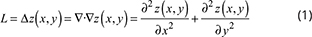
where x and y are the two spatial coordinates in the grid. To compute the Laplacian map, the operator is simply applied to all z in the geological surface producing a Laplacian map, with higher values relating to areas with more variation in the surface.
Transfer functions
To select areas with geologically relevant features, and to suppress the effect of unwanted simulation artifacts in the surface, a transfer function f(L) must be constructed that provides a probability drawing for the current location (x,y) as a function of the Laplacian.
A basis probability level P0 is first set in INPOX. P0 ensures that all areas of the surface have some probability of being drawn and that a desired fraction of the surface is drawn. For instance, if 5% of the surface should be drawn, P0= 0.05 is selected. In the case that, f(L) = P0, the result will be a random selection from a uniform distribution. To manipulate the basis probability, a series of probability functions (f1 (L), f2 (L), f3 (L),…) can be introduced that either increases or decreases the basis probability depending on the Laplacian.
Madsen et al. (2021b) and Enemark et al. (2023) argue that major changes in the elevation of a geological surface in manual interpretation models are related to geologically relevant features. This is argued since variations in elevation mainly arise due to active choices made by the interpreter, for example, when mapping rivers, buried valleys and faults. We introduce f1(L), which increases the probability of drawing a point from the surface as a function of the Laplacian L:

where CP0 is the maximum probability added to P0 and thereby sets importance of the informed point retrieval in contrast to the base level. g is the maximum derivative of f1 (L) with respect to L. L0 is a reference Laplacian and AL0 is the value of L where the steepest rise of f1 (L) occurs. A and g thereby define how quickly and how abruptly f(L) becomes (1+C)P0 rather than P0 when L increases. A graphical representation of f1 (L) can be seen in Fig. 1 (cyan shading, left hand side).

Fig. 1 Proposed transfer function f (L) in INPOX. The red line shows the probability (on the y-axis) as a function of ∆z (on the x-axis). The parameter B divides the values where f1 (L) and f2 (L) are used, shown by cyan and purple shading, respectively. Other parameters are explained in the main text.
Mathematical interpolation of geological point information results in spatial continuous surfaces. Hence, larger discontinuities can stem from either an active choice made by the modeller (e.g. introducing faults) or from the interpolation routines (e.g. using a limited neighbourhood of points locally instead of all points to make the algorithms more computationally feasible). In a system where there are no faults mapped or the Laplacian is significantly different than the faults, a second function f2(L) can be designed to reduce the base probability and minimise the effect of interpolation artifacts:
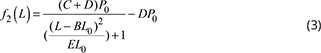
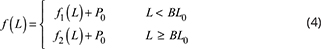
where DP0 is the maximum probability subtracted from P0 , and ELO functions as a dampener going from (1+C)P0 to (1−D)P0. BL0 is the Laplacian defining the switch between domain f1 (L) and f2 (L). A graphical representation of f2 (L) can be seen in the purple part of Fig. 1. In INPOX, the following transfer function is chosen as a combination of f1 (L) (eq. 2) and f2 (L) (eq. 3) with BLO as the separation criteria between two:
Random point retrieval
Once a PM is constructed, the task of drawing the points is trivial. Firstly, the PM is scaled such that the average probability of the entire grid becomes P0. A random map (RM) of similar size to the PM is constructed with values from an uncorrelated uniform distribution between 0 and 1. At each location where the RM value is lower than the PM value, a point is extracted from the surface grid.
Validation using synthetic data
A synthetic reference (surface) model is created (Fig. 2A) with different features that need to be emphasised in the point extraction. At X = 50 and Y = 75, a square is placed that is highly discontinuous with the surrounding surface, while the other features are less discontinuous. The LM is calculated from the reference model and is presented in Fig. 2B. Figure 2C shows two different transfer functions (T1 and T2) to translate the LM into PMs as well as a transfer function where f(L) = P0 (red dotted line) that enables a comparison to random point retrieval (T3, orange line). For T1 (blue line), we treat all changes in the surface as relevant information and emphasise the full spectrum of Laplacians found in Fig. 2B. For T2 (red line), we treat the highly discontinuous square as an interpolation artifact, and only values < 10 are emphasised while values > 10 are suppressed. The parameterisation of each transfer function is presented in Table 1. Three PMs are obtained by applying the three transfer functions. The results are shown in Fig. 2D, H, L, where it is clearly visible that changes in elevation are reproduced using the INPOX strategy and that different points are subsequently drawn based on these probabilities (Fig. 2E, I, M). In the third column (Fig. 2F, J, N), the points are linearly interpolated to create a new surface. The biggest difference between T1 and T2 and the uniform draw (T3) is the lack of dark red and black areas in T3 and thus a lack of structural information and a smoother output surface. Between T1 and T2, the square is more clearly defined in T1 as significantly more points were drawn to help define its shape. The Mean Absolute Deviation (MAD) is calculated in all cases. The MAD confirms the visual validation as T1 and T2 interpolations are closer to the reference model than a uniform draw. Thus, the extracted points carry more of the structurally important information for recreating the reference model. The MAD for T2 is higher than T1 because the suppression of the square extends the difference to the reference model at that location.

Fig. 2 Results from the synthetic case study. A: the reference model. B: the corresponding Laplacians. C: the transfer functions (T1, T2 and T3) used in the experiment. Results are arranged by transfer functions. T1: emphasises all large Laplacians. T2: emphasises all large Laplacians while downplaying the square. T3: uses a uniform distribution. Each row contains: a probability map (D, H, L); a single draw of point extraction (E, I, M); a linear interpolation of the drawn points (F, J, N), 100 repeats of drawing 500 points and interpolating (G, K, O). The Mean Absolute Deviation (MAD) is shown for each interpolation. On average 500 points are drawn from the three probability maps, but the number of points drawn in a single realisation varies as shown in panels E, I and M.
To ensure that these results did not arise because of a fluke draw, we repeat the experiment of drawing a set of points from the PM and interpolating between these 100 times to form a series of new surfaces. The average surface for each transfer function (displayed in Fig. 2G, K, O) confirms that T1 most accurately recreates the reference model on average, while T2 recreates the reference model while downplaying the significance of the square.
To assess the effect of the number of points being drawn in INPOX, we repeat the experiment, generating 100 surfaces from 100 set of points at various basis draw probabilities (here denoted as the draw percentage) of the total grid size. Figure 3 shows the results for draw percentages in the interval between 1% and 13% of the surface being extracted, including the experiment shown in Fig. 2G, K, O that corresponds to a draw percentage approximating 5%. In general, as the draw percentage increases, the informed point retrievals from T1 and T2 decrease the MAD significantly more than T3. At approximately 3%, there are similar levels of MAD, and for very sparse data extraction (< 3%), the pattern is reversed, such that the uniform distribution outperforms T1 and T2. Because the informed extraction tends to cluster the drawn points, some areas may end up with a very low density of points when only a few points are extracted, which makes it difficult to recreate the surface in these areas. In contrast, the uniform extraction always secures an evenly spatial distribution of drawn points and is more robust in cases where data extraction is sparse.

Fig. 3 MAD for 100 point extractions and subsequent interpolations calculated as a function of draw percentage for the three transfer functions T1, T2 and T3. The experiment run in Fig. 2 is shown as a vertical black dotted line.
Naturally, these numbers vary depending on the choice of reference model and transfer function and should not be used directly as decisive indicators of where INPOX is a relevant point-extraction strategy. Instead, in a broader sense, these results indicate that INPOX can be a relevant strategy when a certain number of points need to be extracted, but some minimum of point draw percentage is needed for the method to be effective.
Demonstration using a real-world application
We apply INPOX on a surface from the Danish national hydrostratigraphic model (FOHM; Fælles Offentlig Hydrostratigrafisk Model). This model was created by correlating and interpolating across multiple local models. This has led to many interpolation artifacts that reside amongst valuable geological features. This is exemplified in Fig. 4A through an excerpt of a Quaternary surface from the FOHM model covering 40.4 km2. A river-like structure passes through an area of the surface that is clearly affected by interpolation artifacts. These artifacts can be seen as round shapes (marked with arrows) due to interpolation distances set in the interpolation algorithm. We apply INPOX to extract points from the surface with the input parameters shown in Table 1 as T4. From the LM (Fig. 4B), we assess that most of the geologically relevant features have Laplacians in the interval of 2 and 4, while the artifacts typically have Laplacians larger than ten but can go down to values around 5. Thus, we set B = 3 and C = 5P0 to emphasise the features and E = 0.8 to ensure that all Laplacians above 5 are downplayed in significance.

Fig. 4 Results from the real-world case study. A: an excerpt from a surface in the Danish national hydrostratigraphic model. B the corresponding Laplacian map. C: 2% draw from the surface using INPOX. D: 20% draw from the surface using INPOX. E: Random point extraction using P0 = 0.02. F: Random point extraction using P0 = 0.20. Geol.: geological. Int.: interpolation.
In Fig. 4C, D, we show the result from a single draw with a draw percentage of 2% and 20%, respectively. They likely represent two extremes in terms of point extraction considering that the total number of interpretation points divided by the surface extent is a 9.9% coverage. In the case of the 2% extraction, the greatest concentration of points occurs along the river-like structure and near the highest elevation peaks in the terrain. Conversely, point density is minimal in the low-lying areas, particularly to the south and west. For the 20% draw, the river-like structure is almost completely drawn out, while the artifacts are still difficult to detect visually. This demonstrates that INPOX does exactly as intended in a real-world setting.
Discussion and outlook
In this study we have suggested a method, INPOX, based on calculating the Laplacians at all locations and defining a suitable transfer function to emphasise and suppress certain structures in the surface. Thus, INPOX, to some extent, makes it possible to reverse engineer the process of geological interpolation by extracting the relevant geological features and making it possible to re-interpolate the information. We have successfully validated and demonstrated the applicability of the method in both a theoretical and practical case where geological features are identified and are able to guide the point extraction while interpolation artifacts are removed.
Obviously, INPOX cannot recreate the exact location of points placed by the geologist during interpretation and thus some of the interpolation information cannot be removed using INPOX. By setting the draw percentage, the user can find a suitable trade-off between (1) removing all interpolation information while removing some geological information or (2) keeping all geological information while keeping some interpolation information. If some geologically relevant points are available from for example borehole information, it is trivial to include these in the draw by setting the draw probability in the PM to 1. Madsen et al. (2021b) suggest using the gradient as a measure to calculate the points that are most relevant for describing the surface. As was the case for the Laplacians, the user would look for areas with a steep gradient. Although the gradient will likely provide a reasonable indication of geologically relevant areas of the model, it is difficult to keep information on sharp transitions in the surface. Our tests, although not shown here, confirm this, as the MAD is always worse when using the gradient approach rather than the Laplacian approach. Since the Laplacian is the divergence of the gradient, it is low where the gradient is steep, and high adjacent to these areas. This is more logical because it is more informative to have points where a surface structure begins and ends rather than having the point information on the decline and then recreating the start and end-points with interpolation.
The design of the transfer function matters for the resulting point extraction. In the current setup, INPOX uses a baseline probability that is manipulated with two separate transfer functions, one with the ability to enhance probability and one being able to decrease probability. As demonstrated, one can easily manipulate the parameters to fit the surface features of interest and problems at hand. Furthermore, since all steps in the algorithm have negligible execution times, even on large surfaces, one can fine-tune the parameters of the transfer function in an iterative process until a satisfactory point-extraction strategy is found. For larger surfaces, it might be necessary to construct region-specific transfer functions, however one could also apply one global conservative transfer function that only suppresses extreme Laplacian values.
It is important to stress that INPOX is not limited either by the specific parameterisation or the applied transfer function. One can freely choose another more specific or intricate transfer function if it provides a mapping between the Laplacian and draw probability. For instance, and not shown here, we adapted a piecewise linear function mimicking the T2 transfer-function to a degree that very similar MAD results could be obtained. To conclude, the practitioner should complete a problem-specific assessment of the (spatial) distribution of Laplacians and then make an informed decision on the transfer-function that makes most sense geologically.
Finally, our results on the effect of the draw percentage indicate that choosing INPOX over any other possible point extraction method, as exemplified with the uniform distribution, follows the well-known ‘no-free-lunch’ theorem (Mosegaard 2012; Shalev-Shwartz & Ben-David 2014). This states that the effectiveness of INPOX will be problem dependent. Thus, in some scenarios it could be better to implement another point extraction strategy. If the surface is rapidly fluctuating between neighbouring points, the entropy is high and the information content between points is little to non-existent. In this case, no point extraction method would be preferable. In general, the basic requirement for INPOX is that spatial correlations exist in the surface and furthermore that the surface curvature relates to geological information or artifacts.
We see two main scenarios where INPOX can be a most valuable tool: (1) when dealing with national models, where quality control is often limited to assessing the behaviour of the surface at local scale through cross-sections or possibly 2D maps of the surface and (2) in areas where models are created using different strategies or operate at different scales depending on the resources available for model creation. Under these circumstances, INPOX can be a valuable tool to homogenise what the points represent between different models and even within a single model.
Acknowledgements
The authors wish to thank Geocenter Denmark and the project DECODE-3D for providing funding for writing the manuscript. The method development was carried out in a consultancy project (Nret 2022–2024) conducted for the Danish Environmental Protection Agency (Miljøstyrelsen).
Additional information
Funding statement
The method was developed during consultancy work for the Danish EPA, while the hours for turning the results into a scientific contribution and writing the manuscript was provided by Geocenter Denmark through the project DECODE3D.
Authors’ contribution
RBM: Conceptualisation, software, investigation, writing – original draft preparation
FAF: Conceptualisation, methodology, software, investigation, writing – reviewing and editing
IM: Conceptualisation, supervision, investigation, writing – reviewing and editing
ASH: Project administration, supervision, writing – reviewing and editing
Additional files
None provided