RESEARCH ARTICLE

Neural network predictions of drawdown from groundwater abstraction in the Egebjerg catchment, Denmark

Mathias Busk Dahl^*1,2, , Troels Norvin Vilhelmsen² , Trine Enemark³ , Thomas Mejer Hansen¹

¹Department of Geoscience, Aarhus University, Aarhus, Denmark; ²NIRAS, Aarhus, Denmark; ³Department of Geosciences and Natural Resource Management, University of Copenhagen, Copenhagen, Denmark

Abstract

Results from numerical simulations play a vital role in the decision process of everyday groundwater management. However, these simulations can be time-consuming for large-scale investigations, and it can be necessary to apply approximate methods instead.

This study investigates the abilities of a neural network to replicate simulated drawdown from groundwater abstraction in a numerical groundwater model of the Egebjerg catchment, Denmark. We follow a generalised methodology that uses the information within the deterministic numerical model to create a training set for the neural network to learn from and extend the method to work in a 3D Danish groundwater model case. We compare the abilities of the trained neural network with the results of conventional computations in terms of speed and accuracy and argue that this approach has the potential to improve decision support for decision-makers within groundwater management.

 

 

Introduction

Groundwater models informed by data on geology and hydrological properties of the subsurface are important tools in groundwater management (Gorelick 1983; Pisinaras et al. 2007; Hadded et al. 2013). These models simulate groundwater flow in the subsurface and are used to investigate the environmental effects of external interventions on the groundwater system, such as the establishment of new abstraction wells.

Dahl et al. (2023) provide an approach for training a neural network to replicate the results of drawdown from an abstraction well as simulated in a MODFLOW model (Harbaugh 2005) with a probabilistic output. The network is trained to model the mapping between a few influential model attributes and simulated drawdown. Once trained, the network carries out this mapping at a speed exceeding 100 times that of conventional MODFLOW simulations. Dahl et al. (2023) make use of a synthetic groundwater model and limit the drawdown predictions to the layer of pumping. Here, we extend the method presented in Dahl et al. (2023) to allow abstraction from multiple suitable model layers and predict drawdown in a full 3D real field-based groundwater model of the Egebjerg catchment, East Jylland, Denmark (approx. 55.9748°N, 9.8129°E to 55.8581°N, 9.9645°E). Predictions from the neural network are compared with MODFLOW simulation results, and we discuss the generalisation potential of the tested method.

Materials and methods

The methodology of this paper is based on that presented by Dahl et al. (2023). Our aim is to generalise and test the method on a Danish groundwater model case and explore its implications for groundwater management. The core idea is to train a neural network to predict drawdown from groundwater abstraction using results and features from a numerical groundwater model to significantly reduce computation times. Whilst the method can generally be applied to most groundwater models, a few site-specific decisions need to be made. Our objective is to make minimal changes to the method to accommodate the new groundwater model. We also aim to expand the method’s capabilities from 2D to a full 3D model by training the neural network with simulated drawdown data from all model layers, which come from wells situated in various aquifers.

All the work is performed on a computer with an 13th Gen Intel Core i9 3.00 GHz processor and 128 GB RAM.

Egebjerg groundwater model

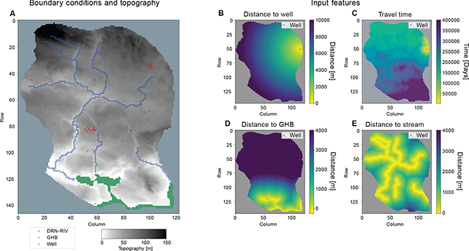
For the Egebjerg catchment, a groundwater flow model has been developed using MODFLOW 6 (Langevin et al. 2017, 2019). This model employs a grid size of 144 × 121 with a 100 × 100 m discretisation across its 14 layers of varying thicknesses (Enemark et al. 2022). Boundary conditions are modelled using the general head boundary package (GHB) for lakes and coastal areas, the recharge package (RCH) for the simulation of groundwater recharge in the top active cells, the drain package (DRN) for simulating stream flow (DRN-RIV in Fig. 1A) and drainage in all top active cells and the well package (WEL) for simulating groundwater abstraction in active wells. Topography and the location of the boundary conditions in the model are visualised in Fig. 1A.

Fig. 1 A visualisation of the Egebjerg model boundary conditions and some of the relevant features for training. A: Streams (blue; DRN-RIV), lakes and fjords (Green et al. 2011) and wells (red; Well) are modelled as boundary conditions shown on top of a topographic map. B–E: Examples of input features to the neural network. DRN-RIV: drain package. GHB: general head boundary package.

The geological layers alternate between sand and clay deposits with a thick chalk aquifer beneath. The downwards extent of the chalk layer is unknown but is assumed to be –550 m below sea level. To simulate layers that pinch out, the vertical pass-through option in MODFLOW 6 is used. This option is applied for cells with a thickness of <0.5 m where flow is distributed downwards to the subsequent active cell.

Data-set construction

The data set for training the neural network consists of sets of target data Y and input features stored in a vector X. Features are related to targets with an unknown function f, such that:

where f is determined through training of the neural network (Gardner & Dorling 1998). Here, the target data Y in Eq. (1) is the simulated drawdown caused by groundwater abstraction in the model. The training data set is created by conducting 1000 simulations. In each simulation, a new well is introduced into the groundwater model. The well’s location is randomly chosen from one of the layers containing water and having a thickness >10 m. Additionally, the pumping rate for the well is drawn randomly from a uniform range spanning 100–5000 m³·day^–1. A single MODFLOW simulation takes 3.2 ± 0.1 s to run. The change in drawdown in each cell caused by the abstraction is saved for the target data.

Dahl et al. (2023) proposed to use a subset of the full information in the model for the input feature vector X. The subset contains 12 influencing features that are generally available in most groundwater models. We extend the method from only observing drawdown from abstraction in a single layer to the full 3D model, where a well can be placed at different depths, and changes in drawdown are predicted for all layers. The features from the Egebjerg groundwater model used for training include the hydraulic head before pumping, distance to well (Fig. 1B), travel time to well (Fig. 1C), distance to head boundary (GHB package; Fig. 1D), distance to stream (DRN package; Fig. 1E), pumping rate, hydraulic conductivity and the logarithmic hydraulic conductivity in the current cell, well location (row, column and layer) and the layer of the current cell. The travel time feature does not represent a specific physical measure but is a proxy of water’s ability to travel to a certain location depending on the distance and flow resistance along the travel route (hydraulic conductivity). The fast-marching algorithm is used to compute these travel times in a 2D plane of the active cells just below topography, as implemented in the scikit-fmm Python extension module (Furtney 2021) and applied in other studies for training machine learning models with simulated data (Thibaut et al. 2021).

Neural network setup

The structure of the neural network consists of an input layer of size 12 (the number of input features), fully connected to three hidden layers, each with 75 neurons as in Dahl et al. (2023). The output layer has two neurons for estimating the mean and standard deviation of a normal distribution representing the drawdown. We apply the Gaussian Error Linear Unit (GELU) activation function (Hendrycks & Gimpel 2016) between the input and hidden layers and a linear activation function between the last hidden layer and the output layer. The Adam algorithm (Kingma & Ba 2014) is used to minimise the loss function, which is defined as the negative log-likelihood of 1D Gaussian distribution. This allows us to interpret the output of the neural network as a Gaussian distribution as describing the drawdown (Dahl et al. 2023). We use the Python libraries Tensorflow and Tensorflow Probability (Abadi et al. 2016; Dillon et al. 2017) for the construction and training of the neural network.

The holding input features of the constructed data set and simulated MODFLOW responses are split 80/20 into a training data set and a validation data set and standardised using a standard scaler. The validation set is withheld from training and used to validate the ongoing training phase to prevent overfitting. During training, if loss improves for the training data but not for the validation data, the neural network is likely overfitting to the training data. We train the network for 1000 epochs and observe a stagnation in loss improvement without encountering overfitting. Additionally, an independent third test data set is constructed from 80 new MODFLOW simulations, separate from the validation data set for performance evaluation.

Results

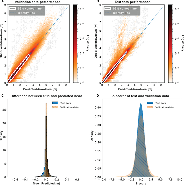
The performances of the trained neural network on the validation and test data are shown in Fig. 2A–B as normalised density plots of MODFLOW simulations (observed drawdown) against mean predictions (predicted drawdown) with a logarithmic colour scale. The sum of all values in the figure adds up to 1. The dashed identity line represents the ideal agreement between MODFLOW simulations and predictions of the neural network. In both data sets, we observe the highest concentrations exactly on the identity line for a drawdown from 0 m and up to c. 3 m. Here lies the highest density region containing 95% of the data marked with the white contour line (Fig 2A–B). In this interval, the data density rapidly decreases as we move away from the line in both directions. For higher values, we observe a shift in the validation data density plot away from the identity line, and the spread increases. Figure 2C shows histograms depicting the differences between true MODFLOW results and predictions within the two data sets, confirming a small error of less than 0.2 m for most differences. Figure 2D displays histograms depicting data set z scores, which quantify the deviation of MODFLOW results x_MOD from the mean prediction μ_NN in terms of standard deviations, σ_NN where,

Fig. 2 The performances of the trained neural network on the validation data set and an independent test data set are shown as density plots A and B. The x-axis represents the predicted mean values of the drawdown, whilst the y-axis represents the observed MODFLOW drawdown. Each square in the figures covers several observations visualised with a normalised logarithmic colour scale. The identity line (blue dashed line) shows the one-to-one agreement between MODFLOW and the network. The white contour line holds 95% of the data within. C shows the difference between the true MODFLOW values and predicted values for both data sets as a probability density histogram. D depicts the distribution of z scores for the validation and test data sets. Brown shading: overlap between test data and validation data sets.

The root mean squared errors between observed and predicted values in Fig. 2A–B are RMSE_vali = 0.19 m and RMSE_test = 0.17 m. The low errors are in good agreement with the observed high density of observations near the identity line and the distribution in Fig. 2C.

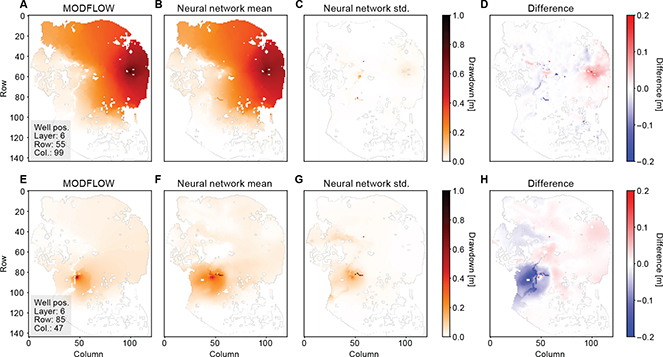
We test the neural network at two different locations outside the original training and validation data sets and compare predictions to MODFLOW results (Fig. 3). In case 1 (Fig. 3A), the well is placed in layer 6 at row 55 and column 99 with a pumping rate of 798 m³·day^–1. The drawdown from the MODFLOW simulation shown in Fig. 3A is compared to the predicted mean and standard deviation from the network (Fig. 3B–C). The difference between MODFLOW and the predicted mean of the network is visualised in Fig. 3D. The network replicates the MODFLOW results well with low differences between the two in most parts of the layer. We observe some areas with larger differences that seem to correlate with locations of boundary conditions such as simulated rivers and other wells. Also, positive values (in Fig. 3D) are observed near the well, indicating that the neural network slightly underestimates the drawdown in this area. These difficult areas are also visible in the standard deviation map of the neural network where locations of other wells are clearly observed.

Fig. 3 Results and comparisons between MODFLOW and the neural network in two test cases. A–D: Case 1. A new well is simulated in layer 6 at row 55 and column 99. The drawdown of the layer above the abstraction layer is visualised for MODFLOW (A), the neural network mean and one standard deviation (B–C) and the difference between MODFLOW and network mean (D). E–H: Case 2. The well is moved to layer 6 at row 85 and column 47, and drawdown is estimated again as in A–D.

In case 2 (Fig. 3E), the well is placed in layer 6 at row 85 and column 47 with a pumping rate of 849 m³·day^–1. Again, MODFLOW results are compared to the neural network (Fig. 3F–G) and subtracted to show the difference (Fig. 3H). The network models the overall extent of the change in layer, though the discrepancy between MODFLOW and network predictions is larger compared to case 1. High differences are especially apparent at the nearby boundary conditions. Again, this difference between results is correlated to the standard deviation map in Fig. 3G, where larger standard deviations are observed.

Predicting the full model drawdown with the network takes 0.60 ± 0.01 s, related to running the neural network and input-feature creation. The run-time is 3.2 ± 0.1 s for MODFLOW simulations.

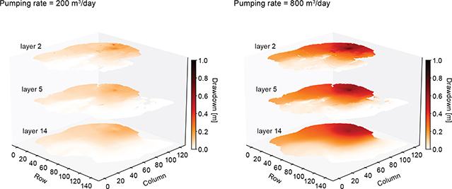
With the pumping rate as an input feature, it is possible to perform tests of pumping series where pumping rates are gradually increased, and drawdown is predicted using the neural network. Figure 4 shows a drawdown in multiple layers for this test where two different pumping rates are used with the same well setup as in case 1 (Fig. 3A–D). Here, all input features are determined once, and only the pumping rate feature is changed for all following network predictions. This reduces the run-time to 0.29 ± 0.04 s per simulation.

Fig. 4 Drawdown in multiple layers predicted with the neural network with the well setup from case 1. Left: the pumping rate is set to 200 m³·day–¹. Right: the pumping rate is increased to 800 m³·day–¹.

Discussion

We have trained a neural network to replicate the results of simulated drawdown using MODFLOW due to groundwater abstraction in the Egebjerg groundwater model, taking the same approach as Dahl et al. (2023) with only a few changes to input features. This demonstrates that the methodology of Dahl et al. (2023) can be generalised, with only minor modifications when applied to new areas. To do this, we extend the method to predict drawdown in all layers and allow the well to be placed in multiple, suitable layers. As a performance test of the neural network on a validation set and an independent test set, results of drawdown from multiple well locations in different layers are presented in Fig. 2. The outcomes reveal a strong agreement between the predictions of the neural network and the results obtained from MODFLOW (Fig. 2A–C), and that a substantial amount of the error can be described with 2 standard deviations (Fig. 2D). The neural network shows a tendency to underestimate higher values of drawdown in Fig. 2A. This is also the case in Dahl et al. (2023) and is likely a consequence of a few high-value observations in the training data compared to the large number of low values available. This could be solved by sampling differently from the training data to favour underrepresented data (Johnson & Khoshgoftaar 2019) or by error-correcting biased predictions (Belitz & Stackelberg 2021).

The case analyses from Fig. 3 show that the network in general replicates the MODFLOW results well. Some difficulties near simulated boundary conditions have a large effect on the predicted mean values. However, these areas also show an increase in the standard deviation maps making them easier to spot and possibly remove or ignore. The standard deviation could potentially act as a verifier of the mean estimate and identify network shortcomings. The accuracy of the network confirms that the applied approach generalises to a Danish case and likely other Danish groundwater models.

The neural network predictions are obtained five times faster than MODFLOW results in the full model. This modest speed-up can be attributed to the efficient run-time of the Egebjerg groundwater model combined with the computation of input features but could potentially be much higher in a model with higher resolution. The neural network, however, provides inherent flexibility, allowing for predictions within specific subareas of the model rather than necessitating computations for the entire model each time, thereby reducing the computational load. Furthermore, for the pumping analysis (Fig. 4), all features, except for the pumping rate, need to be computed only once. This results in subsequent network simulations being 11 times more efficient than those using MODFLOW. Such an analysis for a subarea of the model could greatly reduce the computational time compared to MODFLOW. The proven speed-up and replication accuracy of the network make it a great addition to decision support tools, for example, during initial screening investigations.

Conclusions

In this study, we have trained a neural network to predict drawdown from groundwater abstraction to test the abilities of the network and the applied approach to generalise to a Danish catchment. We extend the approach to the full 3D model to increase user flexibility and general applicability with only a few modifications to input features and network setup. We find a good agreement between MODFLOW results and network predictions and show that areas with high disagreement correlate well with larger network standard deviations. The neural network offers a 5-time speed-up compared to MODFLOW runtime for a single simulation and 11-time speed-up in pumping analysis tests with multiple model runs where input features are only calculated once. Furthermore, the network is flexible and can be limited to predict changes in subareas of the model reducing the number of computations required.

We conclude that the applied approach generalises well to the Danish groundwater model, and that the trained network has potential as a decision support tool.

Acknowledgements

The authors would like to acknowledge Innovation Fund Denmark for funding this project. The authors would also like to thank Robin Thibaut and two anonymous reviewers for a constructive review process that improved the quality of this paper. And a special thanks to handling editor, Hyojin Kim.

Additional information

Author contributions

MD: Conceptualisation, Code Development, Investigation, Methodology, Validation, Visualisation, Writing – Original Draft, Writing – Review & Editing. TV: Conceptualisation, Methodology, Validation, Supervision, Writing – Review & Editing. TE: Code Development, Model Creation, Writing – Review & Editing. TH: Conceptualisation, Methodology, Validation, Supervision, Funding Acquisition, Writing – Review & Editing.

Additional files

Data and code available at https://github.com/MathiasBusk/HYDROSIM_Egebjerg.

References

Abadi, M. et al. 2016: Tensorflow: Large-scale machine learning on heterogeneous distributed systems. arXiv preprint arXiv:1603.04467. https://doi.org/10.48550/arXiv.1603.04467

Belitz, K. & Stackelberg, P.E. 2021: Evaluation of six methods for correcting bias in estimates from ensemble tree machine learning regression models. Environmental Modelling & Software 139, 105006. https://doi.org/10.1016/j.envsoft.2021.105006

Dahl, M.B., Vilhelmsen, T.N., Bach, T. & Hansen, T.M. 2023: Hydraulic head change predictions in groundwater models using a probabilistic neural network. Frontiers in Water 5. https://doi.org/10.3389/frwa.2023.1028922

Dillon, J.V. et al. 2017: Tensorflow distributions. arXiv preprint arXiv:1711.10604. https://doi.org/10.48550/arXiv.1711.10604

Enemark, T., Andersen, L.T., Høyer, A.-S., Jensen, K.H., Kidmose, J., Sandersen, P.B.E. & Sonnenborg, T.O. 2022: The influence of layer and voxel geological modelling strategy on groundwater modelling results. Hydrogeology Journal 30(2), 617–635. https://doi.org/10.1007/s10040-021-02442-9

Furtney, J. 2021: Scikit-fmm: The fast marching method for Python. https://github.com/scikit-fmm/scikit-fmm (accessed June 2023).

Gardner, M.W. & Dorling, S.R. 1998: Artificial neural networks (the multilayer perceptron) – A review of applications in the atmospheric sciences. Atmospheric Environment 32, 2627–2636. https://doi.org/10.1016/S1352-2310(97)00447-0

Gorelick, S.M. 1983: A review of distributed parameter groundwater management modeling methods. Water Resources Research 19, 305–319. https://doi.org/10.1029/WR019i002p00305

Green, T.R., Taniguchi, M., Kooi, H., Gurdak, J.J., Allen, D.M., Hiscock, K.M., Treidel, H. & Aureli, A. 2011: Beneath the surface of global change: Impacts of climate change on groundwater. Journal of Hydrology 405(3), 532–560. https://doi.org/10.1016/j.jhydrol.2011.05.002

Hadded, R., Nouiri, I., Alshihabi, O., Mamann, J., Huber, M., Laghouane, A., Yahiaoui, H. & Tarhouni, J. 2013: A decision support system to manage the groundwater of the Zeuss Koutine Aquifer using the WEAP-MODFLOW framework. Water Resources Management 27, 1981–2000. https://doi.org/10.1007/s11269-013-0266-7

Harbaugh, A.W. 2005: MODFLOW-2005, The U.S. Geological Survey modular ground-water model — the ground-water flow process: U.S. Geological Survey Techniques and Methods 6-A16. USGS. https://doi.org/10.3133/tm6A16

Hendrycks, D. & Gimpel, K. 2016: Gaussian error linear units (gelus). arXiv preprint arXiv:1606.08415. https://doi.org/10.48550/arXiv.1606.08415

Kingma, D.P. & Ba, J. 2014: Adam: A method for stochastic optimization. arXiv preprint arXiv:1412.6980. https://doi.org/10.48550/arXiv.1412.6980

Johnson, J.M. & Khoshgoftaar, T.M. 2019: Survey on deep learning with class imbalance. Journal of Big Data 6(1), 27. https://doi.org/10.1186/s40537-019-0192-5

Kingma, D.P. & Ba, J. 2014: Adam: A method for stochastic optimization. arXiv Preprint arXiv:1412.6980.

Langevin, C.D., Hughes, J.D., Banta, E.R., Niswonger, R.G., Panday, S. & Provost, A.M. 2017: Documentation for the MODFLOW 6 Groundwater Flow Model. Report. U.S. Geological Survey Techniques and Methods 6-A55. http://pubs.er.usgs.gov/publication/tm6A55 (accessed June 2023).

Langevin, C., Hughes, J., Banta, E., Provost, A., Niswonger, R. & Panday, S. 2019: MODFLOW 6 Modular Hydrologic Model Version 6.1.0. U.S. Geological Survey Software. https://doi.org/10.5066/F76Q1VQV

Pisinaras, V., Petalas, C., Tsihrintzis, V.A. & Zagana, E. 2007: A groundwater flow model for water resources management in the Ismarida plain, North Greece. Environmental Modeling & Assessment 12(2), 75–89. https://doi.org/10.1007/s10666-006-9040-z

Thibaut, R., Laloy, E. & Hermans, T. 2021: A new framework for experimental design using Bayesian Evidential Learning: The case of well-head protection area. Journal of Hydrology 603, 126903. https://doi.org/10.1016/j.jhydrol.2021.126903