RESEARCH ARTICLE
Sea-level rise in Denmark: paleo context, recent projections and policy implications
William Colgan*1 , Hans Jørgen Henriksen1
 , Ole Bennike2
 , Sofia Ribeiro1
 , Marie Keiding1
 , Ida Karlsson Seidenfaden1
 , Morten Graversgaard3
 , Anne Gravsholt Busck4
 , Mikkel Fruergaard3
 , Michael Helt Knudsen4
 , John Hopper1
 , Torben Sonnenborg1
 , Maria Rebekka Skjerbæk1, Anders Anker Bjørk4
 , Holger Steffen5
 , Lev Tarasov6, R. Steven Nerem7
 , Kristian K. Kjeldsen1
1Geological Survey of Denmark and Greenland (GEUS), Copenhagen, Denmark. 2Geological Survey of Denmark and Greenland (GEUS), Aarhus, Denmark. 3Aarhus University, Aarhus, Denmark. 4University of Copenhagen, Copenhagen, Denmark. 5Lantmäteriet, Gävle, Sweden. 6Memorial University of Newfoundland, Saint John’s, Canada. 7University of Colorado, Boulder, USA
Citation: Colgan et al. 2022: GEUS Bulletin 49. 8315. https://doi.org/10.34194/geusb.v49.8315
Copyright: GEUS Bulletin is an open access, peer-reviewed journal published by the Geological Survey of Denmark and Greenland (GEUS). This article is distributed under a CC-BY 4.0 licence, permitting free redistribution, and reproduction for any purpose, even commercial, provided proper citation of the original work. Author(s) retain copyright.
Received: 30 Mar 2022; Accepted: 10 Aug 2022; Published: 05 Oct 2022
Competing interests and funding: The authors declare no competing interests.
This work is supported by the Geocenter Denmark project ‘Sea-level rise and coastal flooding in Denmark: past, future, and policy’, with Geocenter partners at the Geological Survey of Denmark and Greenland, the Department of Geoscience at Aarhus University and the Department of Geosciences and Natural Resource Management at the University of Copenhagen.
*Correspondence: wic@geus.dk
Keywords: projection, Denmark, coast, sea level, climate scenario
Abbreviations:
AR6: Sixth Assessment Report
CMIP6: Coupled Model Intercomparison Project Phase 6
DVR90: 1990 Danish Vertical Reference System
IPCC: Intergovernmental Panel on Climate Change
MIS: Marine Isotope Stage
PSMSL: Permanent Service for Mean Sea Level
RCP: Representative Concentration Pathway
SSP: Shared Socioeconomic Pathway
Edited by: Marit-Solveig Seidenkrantz (Aarhus University, Denmark)
Reviewed by: three anonymous reviewers
Abstract
We present the most recent Intergovernmental Panel on Climate Change Sixth Assessment Report (AR6) sea-level projections for four Danish cities (Aarhus, Copenhagen, Esbjerg and Hirtshals) under the Shared Socioeconomic Pathway (SSP) family of climate scenarios. These sea-level changes projected over the next century are up to an order of magnitude larger than those observed over the previous century. At these cities, year 2150 sea-level changes of between 29 and 55 cm are projected under the very low emissions scenario (SSP1-1.9), whilst changes of between 99 and 123 cm are projected under the very high emissions scenario (SSP5-8.5). These differences highlight the potentially significant impact of remaining opportunities for climate change mitigation. Due to this increase in mean sea level, the mean recurrence time between historically extreme events is expected to decrease. Under the very high emissions scenario, the historical 100-year storm flood event will become a 1- to 5-year event at most Danish harbours by 2100. There is considerable uncertainty associated with these sea-level projections, primarily driven by uncertainty in the future evolution of the Antarctic ice sheet and future sterodynamic changes in ocean volume. The AR6 characterises collapse of the West Antarctic ice sheet as a low-probability but high-impact event that could cause several metres of sea-level rise around Denmark by 2150. In climate adaptation policy, the scientific landscape is shifting fast. There has been a tremendous proliferation of diverse sea-level projections in recent years, with the most relevant planning target for Denmark increasing c. 50 cm in the past two decades. Translating sea-level rise projections into planning targets requires value judgments about acceptable sea-level risk that depend on local geography, planning timeline and climate pathway. This highlights the need for an overarching national sea-level adaptation plan to ensure municipal plans conform to risk and action standards.
Introduction
Future sea-level rise, which threatens coastal populations, ecosystems and infrastructures around the world, is highly dependent on society’s choice of future climate pathway (Nauels et al. 2017). Denmark is a relatively low-lying nation — approximately 24% of the country lies within 10 m of sea level — with over 7000 km of coastline (Fig. 1). Presently, approximately 17% of the Danish population lives within 6 m of sea level (Fryd & Jørgensen 2020). This proportion is expected to increase with future population growth focused in coastal cities. The Danish coastline is dynamic and has been dramatically shaped by changes in sea level and sediment transport over the past 2000 years. In northern Jylland, at Skagen, relative sea level has fallen c. 4 m in the past two millennia (Hauerbach 1992; Clemmensen et al. 2001). In central Denmark, near Aarhus, as well as offshore in Kattegat and Øresund, relative sea level has fallen <1 m during the past 2000 years (Bennike et al. 2012, 2021; Clemmensen et al. 2012; Hede et al. 2015). In western Jylland, near Esbjerg, however, relative sea level has conversely risen c. 1.5 m during the same time (Gehrels et al. 2006; Szkornik et al. 2008). These contrasting relative sea-level changes, reconstructed over the past two millennia, primarily reflect spatial variations in the glacial isostatic adjustment of Earth’s crust associated with deglaciation of the Scandinavian ice sheet. On longer timescales, the magnitude of sea-level change is even larger, reflecting absolute increases in ocean volume and elevation associated with the deglaciation of land ice. Reconstructed sea-level curves indicate >30 m of local sea-level rise at several Danish sites during the mid-Holocene, between 12 000 and 6000 years ago (Bennike & Jensen 2011; Bennike et al. 2012, 2019, 2021). Coastal currents and associated sediment transport around Denmark play a major role in shaping the present-day shoreline (Kabuth et al. 2014). This underlines a complex history of sea-level change and shoreline position in Denmark.
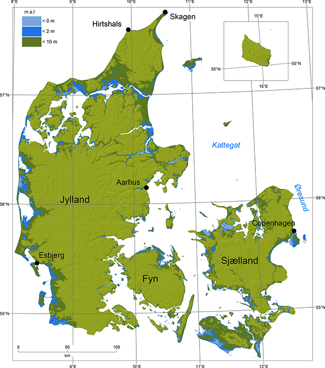
Fig. 1 Overview map of Denmark with place names referred to in the text. Shaded areas designate areas below specified elevations, regardless of whether they have a direct connection to the ocean. This highlights potentially vulnerable areas, should the coastal barrier be breached. The digital elevation map is obtained from the Danish Agency for Data Supply and Infrastructure.
Global sea level is now once again highly dynamic and increasing, in response to anthropogenic climate change. The rate of 21st century sea-level rise is expected to be faster than that for previous warm Holocene intervals, such as the Medieval Warm Period (c. 1000 to 1300 CE) and the Holocene Thermal Maximum (c. 6000 to 4000 BCE; Gehrels & Shennan 2015; Kaufman et al. 2020). Paleo studies also infer a consistently high sensitivity of global sea-level rise to atmospheric warming (Levermann et al. 2013). Specifically, global sea level was at least 6 m higher than present day during the last interglacial (Eemian; Marine Isotope Stage (MIS) 5e) when atmospheric temperatures were at least 1°C warmer than pre-industrial temperatures (Dutton et al. 2015). The rate of forthcoming Anthropocene sea-level rise may be comparable to some of the fastest periods of sea-level rise in the past 12 000 years (Weaver et al. 2003). Since 1993, global mean sea level has already risen 8 ± 1 cm (WCRP Global Sea Level Budget Group 2018). An acceleration in sea-level rise since 1993 is now readily detectable within the global satellite altimetry record, as well as within North Sea tide gauge data (Nerem et al. 2018; Steffelbauer et al. 2022). There is tremendous spatial variability in recent vertical land motion and sea-level change across Europe (Fig. 2). There is a pronounced east–west trend in sea-level change across Scandinavia, with sea levels in the Gulf of Bothnia rising twice as fast as those in the North Sea (Colgan et al. 2019).
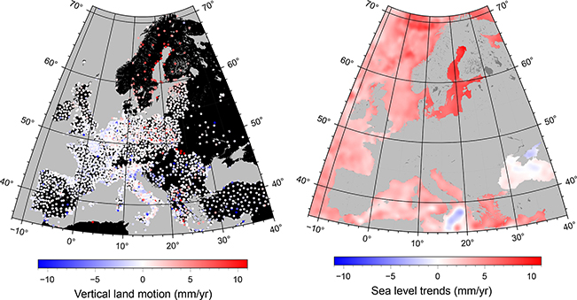
Fig. 2 Trends in European ocean and land elevation between January 1993 and December 2020. Left: Vertical land motion trend observed at fixed global positioning system sites (updated from Hammond et al. 2021). Right: Sea-level elevation trend observed from satellite radar altimetry (updated from Nerem et al. 2018).
The processes influencing recent and future sea-level changes at a specific city are complex. They include larger-scale processes, such as the transfer of land ice into the ocean, the thermal expansion of seawater and shifts in oceanic and atmospheric currents, as well as smaller-scale processes, such as vertical land motion and the redistribution of water masses (Nauels et al. 2017). Consequently, projected sea-level changes are globally non-uniform, and they vary from city to city (Jevrejeva et al. 2016). Here, we examine both the instrumental record of observed sea-level change and the sea-level change projected by the Intergovernmental Panel on Climate Change (IPCC) Sixth Assessment Report (AR6), at four Danish cities (Holgate et al. 2013; Fox-Kemper et al. 2021). Our aim is to provide policy-relevant insight on local sea-level budgets that resolve all sea-level components, and their associated uncertainties, under the IPCC AR6 Shared Socioeconomic Pathway (SSP) climate scenarios. These scenarios have five fundamental storylines (O’Neill et al. 2020; Fig. 3). SSP1 characterises a ‘sustainable’ future with very low to low emissions and low challenges associated with climate change adaptation and mitigation. SSP2 characterises a ‘middle of the road’ future with intermediate emissions and challenges. SSP3 characterises a ‘rocky road’ with high emissions and challenges associated with growing regional rivalries. SSP4 characterises a future of ‘inequality’ and high emissions arising from clear regional pathways dominated by adaptation challenges. Finally, SSP5 characterises a future taking the fast road of ‘fossil-fuel development’ and very high emissions dominated by mitigation challenges. These storylines incorporate broad assumptions about underlying social demographics and offer a wide range of future climates, including multiple alternative pathways to the same climate forcing (Fig. 3; Meinshausen et al. 2020). The differences in sea-level rise projected under this range of scenarios highlight the significant impact of remaining opportunities for climate change mitigation.
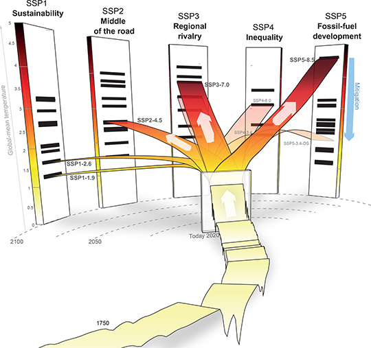
Fig. 3 The five SSP storylines with global-mean temperature illustrated relative to pre-industrial levels. The historical temperatures branch into the respective five SSP scenarios over the 21st century. The small black horizontal bars on the 2100 pillars for each SSP indicate illustrative temperature levels. The opaque bands over the 21st century indicate the five SSP scenarios SSP1-1.9, SSP1-2.6, SSP2-4.5, SSP3-7.0 and SSP5-8.5 that are explored in this study. Other scenarios (SSP4-6.0, SSP4-3.4 and SSP5-3.4-OS) are not explored in this study. Modified slightly from Meinshausen et al. (2020).
Methods
We employ sea-level projections made available through the IPCC AR6 Sea-Level Projection Tool at https://sealevel.nasa.gov/ipcc-ar6-sea-level-projection-tool (Fox-Kemper et al. 2021; Garner et al. 2021). The AR6 makes sea-level projections for Permanent Service for Mean Sea Level (PSMSL) reporting stations around the world (Holgate et al. 2013). Within Denmark, four PSMSL stations are available: Aarhus (station 76), Esbjerg (station 80), Copenhagen (station 82) and Hirtshals (station 89; Fig. 1). AR6 selected these four stations from the 14 available PSMSL stations within Denmark to ensure globally homogeneous coverage that is representative of spatial variations in vertical land motion (Hansen 2018). At each of these four stations, the sea-level projection is estimated every 10 years between 2020 and 2150 using a local multi-component sea-level budget. The six components of this budget are (1) sterodynamic ocean-volume changes, (2) the Antarctic ice sheet, (3) the Greenland ice sheet, (4) mountain glaciers, (5) vertical land motion and (6) changes in land-water storage. Sea-level projections are made under five illustrative SSP scenarios: SSP1-1.9 (very low emissions), SSP1-2.6 (low emissions), SSP2-4.5 (intermediate emissions), SSP3-7.0 (high emissions) and SSP5-8.5 (very high emissions).
The AR6 provides relative sea-level projections as height changes relative to a 2005 baseline. We translate these sea-level changes to a 1990 baseline by fitting a second-order polynomial curve to the mean annual sea-level elevation observed at each PSMSL station between 1900 and 2020. Our polynomial curve fitting ignores years with no data. Our polynomial approach deviates from the prevailing Danish Coastal Authority approach of applying linear best fit to historical data, which may cause small discrepancies in reported historical sea-level change (Ditlevsen et al. 2019). We estimate the change in sea-level baseline between 1990 and 2005 by differencing the respective annual values of our polynomial fit. This yields 2005 to 1990 baseline corrections to the AR6 relative sea-level changes of +0.2 cm at Hirtshals, +1.6 cm at Aarhus, +2.0 cm at Copenhagen and +2.6 cm at Esbjerg (Fig. 4). Translating these relative projections into absolute sea-level elevation in the standard 1990 Danish Vertical Reference system (DVR90) requires a further correction that reflects the offset between the 1990 baseline sea level and the reported DVR90 elevation for each station (Table 1). Aside from using a polynomial, rather than linear best fit, this DVR90 conversion conforms to the Danish Coastal Authority approach for linking local DVR90 datum to local sea-level elevation (Kystdirektoratet 2018).
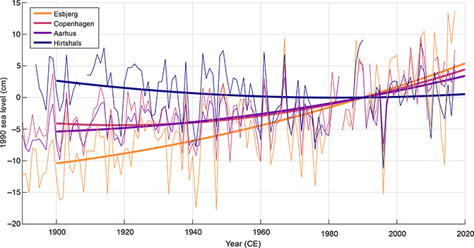
Fig. 4 Permanent Service for Mean Sea Level (PSMSL) records of sea-level elevation relative to 1900 at four Danish sites (Holgate et al. 2013). Thick lines are second-order polynomial fits that ignore missing data. These polynomial fits are used to correct the 2005 baseline of AR6 sea-level projections to the 1990 baseline of the Danish Vertical Reference System (DVR90).
Results
The PSMSL records at Aarhus, Esbjerg, Copenhagen and Hirtshals reveals a spatially complex pattern of sea-level change over the 1900–2020 period, even within the relatively limited size of Denmark (Fig. 4). Hirtshals and Esbjerg are clear end members for this sea-level change. At Hirtshals, the relative sea level has fallen very slightly since 1900 (–2 ± 2 cm). At Esbjerg, by contrast, the relative sea level has increased sharply since 1900 (+16 ± 2 cm). The distance between these two PSMSL sites is only c. 255 km. This sharp gradient in recent sea-level change is ultimately associated with the complex pattern of glacial isostatic adjustment following the relatively rapid deglaciation of the Scandinavian ice sheet, with Denmark becoming ice-free c. 16 000 years ago (Houmark-Nielsen & Kjær 2003). At Esbjerg, the Earth’s crust is presently subsiding due to the collapse of the crustal forebulge that once ringed the Scandinavian ice sheet, whilst at Hirtshals, the crust is presently rebounding upwards due to ice unloading (Steffen & Wu 2011). The post-1900 sea-level changes at Copenhagen and Aarhus, both +9 ± 2 cm, lie between these end members.
The inter-city differences in observed sea-level change are also generally reflected in the projected sea-level changes (Fig. 5). There can be, however, a non-physical inflection of observed and projected sea-level changes at the year 2020 observation-model transition. This is perhaps most evident at Hirtshals and likely results from vertical land motion not being treated consistently between observations and projections. Under all climate scenarios, the projected sea-level rise is systematically c. 25 cm higher at Esbjerg than at Hirtshals. This difference in sea-level rise associated with geography, however, is clearly smaller than the c. 70 cm difference associated with choice of climate scenario. Simply put, whilst presently non-trivial, with increasing warming, the vertical land motion component of sea-level change becomes small relative to the thermal expansion and cryospheric contributions to sea-level change. For example, at Aarhus, the year 2150 sea-level rise ranges from 45 (8–90) cm under the very low emissions scenario (SSP1-1.19) to 115 (69–176) cm under the very high emissions scenario (SSP5-8.5; Table 2). Here, the 90% confidence intervals indicate that there is a 95% chance that sea-level rise will be less than 90 cm under SSP1-1.9 and less than 176 cm under SSP5-8.5. Clearly, however, the sea-level changes observed over the past century are an order of magnitude smaller than the sea-level changes expected over the next century.
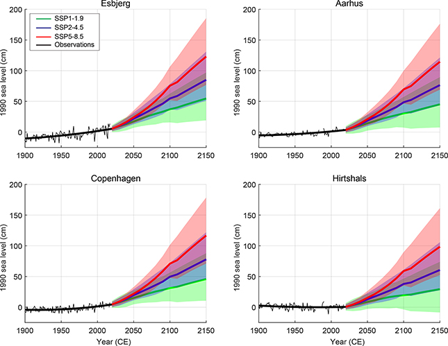
Fig. 5 Permanent Service for Mean Sea Level (PSMSL) observed sea-level change (1900-2020; Holgate et al. 2013) and AR6 projected sea-level change (2020–2150; Fox-Kemper et al. 2021) at four Danish cities, expressed relative to a 1990 baseline. Shaded areas denote the uncertainty associated with each projection. The SSP1-2.6 and SSP3-7.0 projections are omitted for clarity but appear tabulated in Table 2. The c. 2100 ‘bumps’ in projections are a known artifact associated with a decrease in available CMIP6 (Coupled Model Intercomparison Project Phase 6) simulations after 2100, in comparison to before 2100.
Table 2 presents summary statistics to explicitly address four distinct elements of planning for sea-level change in Denmark. First, as discussed earlier, projected sea-level rise varies by location. Second, projected sea-level rise varies by year, or planning timeline, of interest. Third, projected sea-level rise varies with the choice of climate scenario. Finally, and perhaps most importantly, interpreting the appreciable 90% confidence uncertainty is ultimately a risk assessment. AR6 assesses the uncertainty associated with its sea-level projections based on ensemble spread, in both higher-complexity simulations and lower-complexity emulations, as well as structured expert judgment. Arguably, the most conservative approach for interpreting an upper-limit metric for sea-level rise planning is pessimistically assuming the very high emissions climate scenario (SSP5-8.5) with the longest timeline (year 2150) and upper limit (95%) of the confidence interval. This yields upper limit metrics of +186 cm at Esbjerg, +179 cm at Copenhagen, +176 cm at Aarhus and +161 cm at Hirtshals. Conversely, the ambition of The Paris Agreement to limit climate change, combined with the need for nearer-term planning targets, can also justify the use of substantially lower planning metrics across Denmark. For example, assuming sea-level changes between +22 and +29 cm across all four cities, in the year 2050 under the SSP1-1.9 very low emissions scenario and 95% upper confidence limit. In short, translating the projections in sea-level rise presented here into planning targets requires making value judgements about the acceptable exposures and vulnerabilities to sea-level hazards that depend on geography, timeline and climate choices.
Discussion
Projection uncertainty
There are two main types of uncertainty associated with the AR6 sea-level projections (Fig. 6). The first type of uncertainty is the climate trajectory associated with the five AR6 climate scenarios: SSP1-1.9 (sustainability, very low emissions), SSP1-2.6 (sustainability, low emissions), SSP2-4.5 (middle of the road, intermediate emissions), SSP3-7.0 (regional rivalry, high emissions) and SSP5-8.5 (fossil-fuel development, very high emissions; O’Neill et al. 2020). These climate scenarios forecast how society’s greenhouse gas emissions may evolve until 2150. Climate scenario uncertainty therefore clearly represents more of a social than physical uncertainty. Generally, however, the differences projected between scenarios highlight the significant impact of remaining opportunities for climate change mitigation. Simply put, society can still avoid substantial future sea-level rise if we can divert from our current high-emissions climate pathway to a low-emissions climate pathway. The second type of uncertainty is the process-level uncertainty associated with each of the six components in the AR6 sea-level budget: (1) sterodynamic ocean-volume changes, (2) Antarctic ice sheet, (3) Greenland ice sheet, (4) mountain glaciers, (5) vertical land motion and (6) changes in global land-water storage. Both the magnitude and uncertainty of these latter two terrestrial processes are relatively small for all climate scenarios. Thus, terrestrial processes are not the main drivers of the sea-level changes projected around Denmark by the AR6. Next, we describe how other components of the sea-level rise budget influence Denmark.
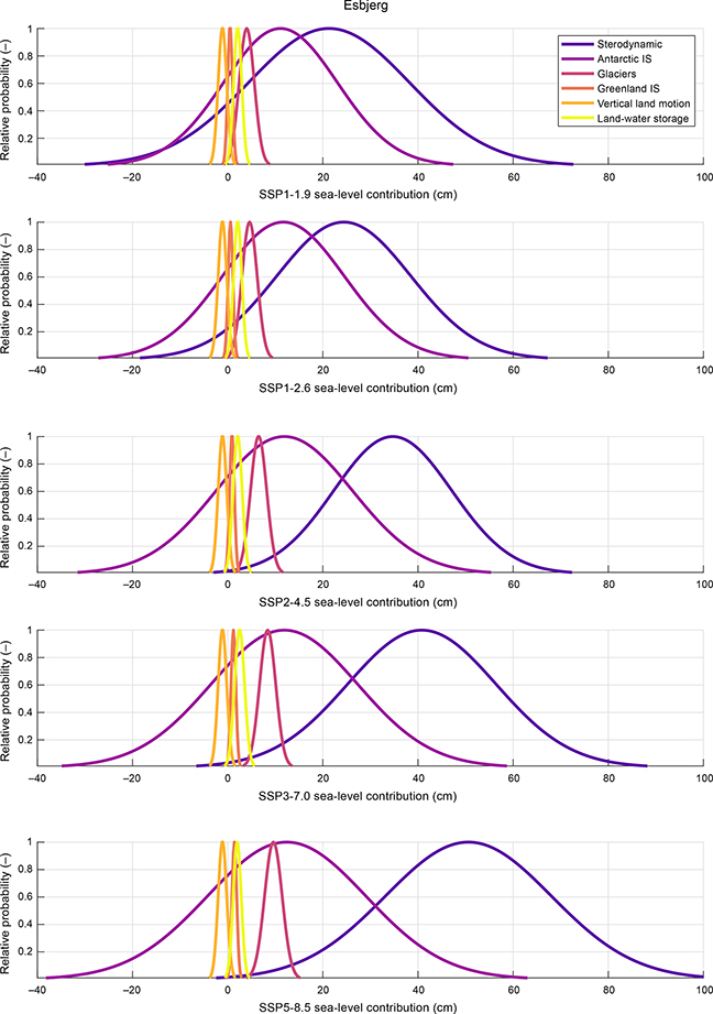
Fig. 6 Relative probability distributions of the six contributing terms for the ‘medium confidence’ year 2150 AR6 sea-level budget at Esbjerg (Fox-Kemper et al. 2021). The six components of sea-level change are shown under the five AR6 climate scenarios. The distributions shown here are broadly representative of other Danish cities.
The Greenland ice sheet contribution and associated uncertainty are an order-of-magnitude smaller than that of mountain glaciers across all five climate scenarios. This is perhaps counter-intuitive, as the Greenland ice sheet is a larger contributor to global mean sea-level rise than mountain glaciers. This apparent inversion, however, is an anticipated local consequence of shifting planetary gravity due to the redistribution of water and ice masses (Larour et al. 2017). Denmark is located within the regional gravitational weakening, and sea-level fall, associated with ice loss from Greenland. This makes the Greenland ice sheet contribution to sea-level rise disproportionately smaller around Denmark, in comparison to the global mean (Colgan et al. 2019). Denmark is conversely located well beyond the analogous regional gravitational weakening associated with Antarctic ice loss and, therefore, receives disproportionately more sea-level rise from the Antarctic, in comparison to the global mean. Danish sea-level projections therefore incorporate substantially more uncertainty associated with Antarctic ice loss, in comparison to Greenland ice loss. Antarctic ice loss, which is a key source of uncertainty in both Danish and global projections, is discussed in Section 4.2.
There is also tremendous uncertainty associated with sterodynamic ocean-volume changes. These are the changes in ocean volume associated with the warming and expansion of ocean water, as well as the dynamic redistribution of ocean mass associated with changing currents. Across all climate scenarios, sterodynamic changes are one of the largest components within the AR6 sea-level budget, accounting for 30–40% of the total global sea-level rise, and within every climate scenario, there is substantial uncertainty (year 2150 standard deviation approximately ± 14 cm across the Danish sites; Fox-Kemper et al. 2021). Whilst the relation between water temperature and water density is well-known, and recent thermal expansion is well-observed, modelling the future thermal expansion of the ocean is challenging due to poor scientific understanding of how atmospheric heat is mixed into the near-surface ocean (Church et al. 1991; Zanna et al. 2019; Marti et al. 2022). So how deep will the ocean warm and expand due to spatially and temporally variable processes of downward heat advection and diffusion? The uppermost 700 m of the oceans has absorbed the vast majority of the anthropogenic climate energy associated with global warming since the industrial revolution, but how will the deeper oceans respond to future forcing? In the AR6 projections, the sterodynamic contribution is relatively large across all climate scenarios, which reflects the substantial future thermal expansion committed by past global warming (Ehlert & Zickfeld 2018).
Ice-sheet collapse
Aside from sterodynamic ocean-volume changes, a second critical source of uncertainty in the AR6 projections is the Antarctic ice sheet contribution to sea-level rise. The projections described in Section 4.1 are regarded as ‘medium confidence’ by the AR6. This is a qualitative term used by the IPCC to convey medium validity based on the type, amount, quality and consistency of data. The AR6 also includes a ‘low confidence’ projection, which, by definition, conveys lower validity from underlying data that incorporates substantially higher near-term contributions from collapsing ice sheets. In comparison to the ‘medium confidence’ projection, which estimates a 5% chance of >230 cm of sea-level rise at Copenhagen in 2150, the ‘low confidence’ projection with additional ice-sheet collapse projects >450 cm at Copenhagen in 2150 (Fig. 7). Whilst the physical mechanisms associated with near-term ice-sheet collapse are qualitatively described, they are difficult to quantify in numerical models (Larour et al. 2021). The likelihood of such low probability, but high impact, events is, therefore, inherently difficult to assess beyond expert elicitation (Bamber et al. 2019).
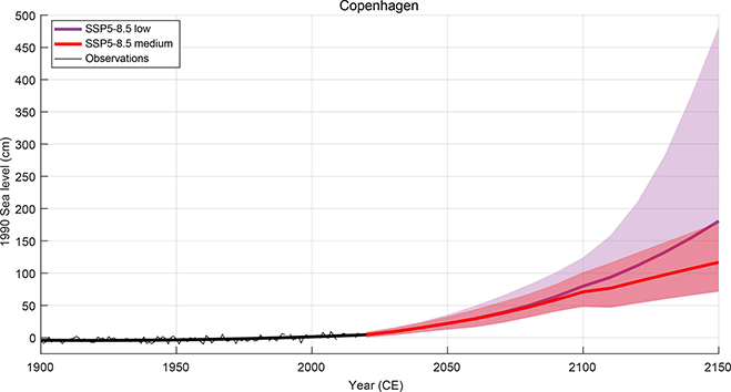
Fig. 7 AR6 SSP5-8.5 projections with (‘low confidence’) and without (‘medium confidence’) ice-sheet collapse at Copenhagen (Fox-Kemper et al. 2021). The projections shown here are broadly representative of other Danish cities.
The primary concern for ice-sheet collapse is the marine ice-sheet instability hypothesis, which fundamentally suggests that the retreat of glaciers grounded below sea level on retrograde bed slopes is irreversible on human time scales (Mercer 1978). For the West Antarctic ice sheet especially, which is largely grounded below sea level, this means that the retreat of major outlet glaciers can initiate a collapse of multi-metre sea-level equivalent over relatively short time scales (Bamber et al. 2009). There are growing observations of glacier retreat, thinning and acceleration that together suggest that a tipping-point threshold has been crossed, and ice-sheet collapse is already underway in the Amundsen Sea sector of West Antarctica (Joughin et al. 2014; Rignot et al. 2014; Voosen 2021). In a recently structured expert judgment from 23 global sea-level researchers, 5% of respondents expected West Antarctica’s sea-level contribution over the 21st century to track a ‘high-end’ (i.e. high emissions) contribution consistent with marine ice-sheet instability (Bamber et al. 2019).
In the longer term, numerical ice-sheet projections under an SSP5-8.5 very high emissions scenario suggest that both the Greenland and Antarctic ice sheets are poised to deliver multi-metre sea-level rise for centuries to come (Fig. 8; Aschwanden et al. 2019; Chambers et al. 2021). More specifically, the ‘high-end’ ensemble members within these projections suggest that complete loss of the Greenland ice sheet (c. 7.2 m sea-level equivalent) and West Antarctic ice sheet (c. 3.3 m sea-level equivalent) is possible by c. 2500 with currently included model processes. This would raise global mean sea level by >10 m in five centuries, which may be up to half the deglaciation rate of meltwater pulse 1A, which occurred c. 14 500 years ago (Weaver et al. 2003; Liu et al. 2016). Whilst recently observed ice-sheet mass loss closely tracks the consensus RCP (Representative Concentration Pathway) 8.5 high emissions projection of the recent IPCC AR5 (The IMBIE Team 2020), there is emerging evidence that numerical ice-sheet simulations systematically underestimate the ice loss observed in the recent past (Aschwanden et al. 2021). Ice-sheet models can suffer from uncertainty associated with boundary conditions, initial conditions, spatial and temporal resolution, parametric calibration and process inclusion. Community assessments derived from an ensemble of ‘best estimate’ models rarely probe these deeper inter-model uncertainties in a systematic fashion (Levermann et al. 2014). Generally, the scientific debate surrounding ice-sheet collapse has now moved beyond whether it is theoretically possible to whether it is realistically possible under sustained very high emissions.
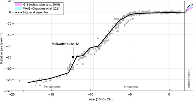
Fig. 8 Reconstruction of global mean sea-level since the Last Glacial Maximum, spanning the latter part of the Pleistocene and the Holocene, with the grey dots representing individual observations and black line representing trend after Fleming et al. (1998). Anthropocene high-emission (RCP8.5/SSP5-8.5) projections of Greenland ice sheet (‘GIS’; Aschwanden et al. 2019) and West Antarctic ice sheet (‘WAIS’; Chambers et al. 2021) collapse are shown, ignoring associated sterodynamic effects, with the ‘high-end’ ensemble member denoted.
Extreme events
Whilst we present and describe forecasted changes in mean sea level under differing climate scenarios, it is important to recall that local sea level can vary substantially on daily timescales due to tidal and storm effects (Wahl et al. 2017; Thompson et al. 2021). The 1872 Baltic storm, which has been characterised as a once in 4500-year event, delivered extreme sea levels that were up to 280 cm above historical mean sea level in south-east Denmark (Clemmensen et al. 2014). Understanding extreme sea-level events, such as high tide or storm flooding, is critical to understand the inherent risk associated with sea-level rise. The risk of an extreme sea-level event is generally characterised by its recurrence interval. Tide gauge records are used to assess the magnitude of historical extreme events, for example characterising the height above mean sea level of the 100-year or 10-year events. As mean sea level around Denmark increases, however, the height of extreme sea-level events will also increase, which effectively decreases historical recurrence intervals (Su et al. 2021).
At Aarhus, the 100-year extreme sea-level event has been estimated as +163 cm above mean sea level, based on tide gauge observations during the 1981–2010 period (Fig. 9; Kystdirektoratet 2018; Thejll et al. 2021). Under the RCP8.5 high-emissions climate scenario, however, increases in mean sea level result in this same sea-level height recurring as a 5-year event during the 2071–2100 period. Su et al. (2021) suggest it will become a 1-year event. In short, sea levels equivalent to the historical 100-year event will occur at least 20 times more frequently during the last decades of the century under the RCP8.5 scenario. As a consequence, the annual duration of high water-level warnings at Aarhus will increase from c. 3 h per year in 1981–2010 to c. 1280 h per year (or c. 15% of the year) in 2071–2100 under the RCP8.5 high-emissions climate scenario median estimates (Thejll et al. 2021). This general pattern, characterised by decreasing extreme event recurrences and increasing duration of water-level warnings, is similar for other cities around Denmark (Kystdirektoratet 2018, 2022). These decreases in recurrence intervals are based on stationary statistics and ignore any changes in recurrence due to potential changes in storminess or seasonal cycle. They simply assume that future flooding events will be a composite of historical-type storm surges overlaid on projected sea-level rise.
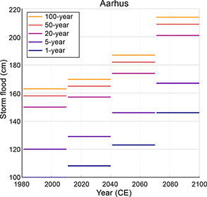
Fig. 9 Storm flood height above mean sea level (cm) for 1-, 5-, 20-, 50- and 100-year recurrence intervals at Aarhus. Calculated over different 30-year climatology periods until 2100 under the RCP8.5 high emissions climate scenario (Kystdirektoratet 2018; Thejll et al. 2021).
The risk presented by these transient extreme sea-level events is currently managed with a variety of hard and soft solutions around Denmark (Fig. 10; Mangor et al. 2017). Hard solutions are engineered constructions of dikes, sluices, sea walls, floodgates and quay–terrain elevation, often with the primary purpose of maintaining the coastline position without any significant changes. Soft solutions typically use nature-based approaches, such as establishing new artificial islands, sand dunes or reefs and sand nourishment and/or revegetation along the coastline, with the primary purpose of reducing flood risk. Both types of solutions can play a key role in protecting existing and future developments and assets from coastal erosion and inundation (Faragó et al. 2018; Fryd & Jørgensen 2019). The choice between various hard and soft coastal management strategies is ultimately dependent on the municipal management strategy, which can range from the high-burden of ‘hold-the-line’ to low-burden of unmitigated retreat, as well as coastal morphology and the dominant coastal processes during extreme sea-level events.
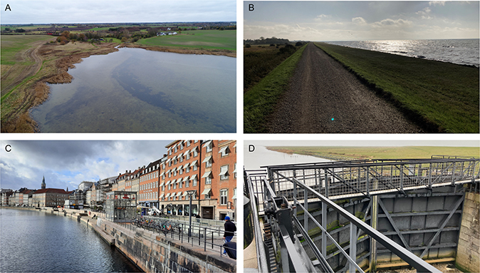
Fig. 10 Diversity of management of options for extreme sea-level events. A: Coastal wetland in Roskilde Fjord, Sjælland. B: Earthen coastal protection dams near Rødby, Sjælland. C: Hardened shoreline at Copenhagen, Sjælland. D: High-water river lock on Ribe Å, Jylland.
Municipal planning
We provide a summary of previously published sea-level projections that are relevant for sea-level rise planning at Copenhagen in Fig. 11. These previous projections, which discount any scenarios of ice-sheet collapse, are collected from studies and assessments published since the 2007 IPCC Fourth Assessment Report (Table 3). All these sea-level projections correspond to a ‘high’ or ‘very-high’ emissions climate-change scenario (i.e. the previously published A1B, RCP8.5 scenarios or SSP5-8.5). The AR6 sea-level projections discussed here are the most recent projections available. Whilst previous IPCC assessments reported sea-level rise projections as tabulated global averages, AR6 now provides city-level sea-level projections. After accounting for the use of differing baseline years, these nine studies suggest that the best estimate, for planning purposes, of sea-level rise at Copenhagen increased c. 25 cm per decade between 2007 and 2021. There is, however, tremendous variability between studies. For example, the Danish Climate Atlas (Thejll et al. 2021) projects 22 cm less sea-level rise in the year 2100 than the AR6 (Fox-Kemper et al. 2021). Additionally, these previous studies do not use the same confidence or uncertainty limits, which can make ‘high’ and ‘low’ estimates not directly comparable (Table 3). This underlines the need to continually update datasets and projections and make these available for planners, stakeholders and policy makers.
| Data label | Study name | Study year | Projection baseline | Projection year | Projection type | Scenario | Low (cm) | Mean (cm) | High (cm) |
| 1 | AR4 | 2007 | 1990 | 2100 | G | A1B +ice sheets | 20 | 41 | 61 |
| 2 | SWIPA2011 | 2011 | 1990 | 2100 | G | A1B | 90 | 125 | 160 |
| 3 | AR5 | 2013 | 1996 | 2100 | G | RCP8.5 | 52 | 74 | 98 |
| 4 | Jevrejeva2016 | 2016 | 2005 | 2100 | C | RCP8.5 (+5°C) | 55 | 96 | 193 |
| 5 | SWIPA2017 | 2017 | 2005 | 2100 | G | RCP8.5 | 46 | 74 | 102 |
| 6 | KlimaAtlas | 2019 | 1996 | 2100 | C | RCP8.5 | 6 | 50 | 94 |
| 7 | Colgan2019 | 2019 | 1925 | 2100 | C | RCP8.5 | 49 | 77 | 105 |
| 8 | SROCC | 2019 | 1996 | 2100 | G | RCP8.5 | 61 | 84 | 110 |
| 9 | AR6 | 2021 | 2005 | 2100 | G | SSP5-8.5 (medium confidence) | 63 | 77 | 101 |
| 9 | AR6 | 2021 | 2005 | 2100 | C | SSP5-8.5 (medium confidence) | 48 | 71 | 102 |
| 9 | AR6 | 2021 | 2005 | 2150 | G | SSP5-8.5 (medium confidence) | 98 | 132 | 188 |
| 9 | AR6 | 2021 | 2005 | 2150 | C | SSP5-8.5 (medium confidence) | 51 | 118 | 230 |
| Data labels correspond to Fig. 11 and literature references below the table. G: global; C: Copenhagen-specific. All studies are graphically depicted relative to a common 1990 baseline sea level in Fig. 4. Data labels refer to the following studies: 1: Meehl et al. (2007). 2: AMAP (2011). 3: Church et al. (2013). 4: Jevrejeva et al. (2016). 5: AMAP (2017). 6: Thejll et al. (2021). 7: Colgan et al. (2019). 8: Oppenheimer et al. (2019). 9: Fox-Kemper et al. (2021). |
|||||||||
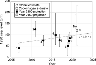
Fig. 11 Previously published sea-level projections of relevance for Copenhagen sea-level rise planning under a high-emissions climate change scenario. All studies expressed relative to 1990 sea level. Data labels are associated with specific previous studies in Table 3. Marker shape indicates global versus Copenhagen-specific projections. Marker colour indicates year 2100 versus 2150 projections. Dashed line denotes the sea-level projection for planning purposes increasing at c. 2.5 cm/yr. The trend shown here is broadly representative of other Danish cities.
There are several reasons for the increasing trend in forecasted sea-level rise. Part of this trend reflects an extension of projections from year 2100 to year 2150 in AR6. As sea level rises through time, longer projections yield larger increases in relative sea level. AR6 projects Copenhagen-specific sea-level rise to be within c. 10% of the global mean projection. This suggests that adopting global projections for Copenhagen-specific planning purposes is generally valid with an additional uncertainty of ± 10% relative to global projections. The shift from more global to more Copenhagen-specific projections over the past decade therefore does not explain the worsening sea-level rise forecast at Copenhagen. We instead suggest that the increasing trend of sea-level rise projections is primarily due to improved process-level understanding of the influence of climate change on sea-level change over time. It is reasonable to expect this trend to continue.
There are diverse sea-level adaptation challenges confronting different coastal municipalities around Denmark. The nature of these challenges depends on city layout and topography, as well as inland hydrological conditions (i.e. groundwater level) or coastal hydrodynamic conditions (i.e. tides and waves; Mangor et al. 2017). For example, a city situated within a fjord is confronted with a different flooding hazard than a city situated along an exposed shoreline. Consequently, the adaptation challenges confronting Danish municipalities span across sea-water flooding, river-water flooding, salt-water intrusion and rising groundwater levels. This highlights the need for site-specific solutions and adaptation strategies. In Denmark, sea-level rise planning has been decentralised since 2008, with at-risk coastal local municipalities each responsible for their own analyses of flood risks and developing prioritised climate change adaptation action plans. Since 2015, EU regulations have also required at-risk coastal municipalities to act to reduce flooding risks (European Parliament 2007).
Madsen et al. (2019) found that whilst Danish municipalities are, indeed, aware that rising sea levels will impact their infrastructure, precise municipal responses often remain poorly defined. Ergo, there is no national requirement to enforce consistent definitions or updates of municipal sea-level rise adaptation plans. This absence of sea-level rise adaptation plan standards creates the possibility for very different risk management and adaptation actions to occur in nearby municipalities with similar coastal geomorphology and coastal processes. It is evident that local adaptation plans must make critical choices, considering both site-specific hydrology challenges and the general issues of geography, timeline, climate choices and acceptable risk level. Arguably, however, there is a pressing need for an overarching common national sea-level adaptation plan to ensure that individual municipal plans conform to some standards in terms of risk analysis using systematically defined vulnerabilities, exposures and hazards.
Conclusions
Here, we review sea-level changes at four Danish cities during both a past instrumental period and a future projection period. Whilst these cities have experienced significant and differing sea-level changes over the instrumental period, the sea-level changes now confronting Denmark over the next two centuries are equivalent, or larger, than the sea-level changes experienced in the past two millennia. In a paleo context, the rate of forthcoming Anthropocene sea-level rise will likely be comparable to some of the fastest periods of sea-level rise during the Holocene, meaning the past c. 12 000 years. Translating the local sea-level rise projections presented here into planning targets, however, is challenging. This requires making value judgments about acceptable vulnerabilities and exposures to sea-level hazards that depend on geography, timeline, societal and climatic pathways and risk level.
The uncertainty associated with society’s 21st century choice of SSP imparts a tremendous uncertainty on local projections of sea-level rise. The differences in sea-level rise projected under the range of scenarios highlight the potentially significant impact of remaining opportunities for climate-change mitigation. Aside from this social uncertainty, across all SSP scenarios, the largest physical uncertainty in projections is associated with the sterodynamic component of sea-level rise. Whilst Denmark is geographically closer to the Greenland ice sheet, uncertainty associated with the Antarctic ice sheet’s response to climate change represents a greater sea-level threat to Denmark. The IPCC scenarios analysed here, however, do not assess the likelihood or impact of rapid ice-sheet collapse. Over longer, multi-centennial, time scales, it is difficult to understate the sea-level threat confronting Denmark associated with ice-sheet collapse. The ‘low-probability high-impact’ scenario of ice-sheet collapse and c. 10 m sea-level rise by 2500 cannot be excluded under higher emission scenarios. Ice-sheet projections suggest that the only way to avoid certain ice-sheet collapse is to avoid a sustained higher emissions climate pathway.
The landscape of sea-level information available to Danish policymakers is shifting fast. Over the past two decades, the most relevant sea-level rise planning threshold for Copenhagen has been increasing at 25 cm per decade. This implies a continual need for updating sea-level projections using the state-of-the-art knowledge and translation of these projections to ensure usability for local stakeholders. There are a variety of hard and soft coastal management strategies already in use in Denmark today. The choice of these strategies is ultimately dependent on both municipal management strategy and coastal morphology or processes. Whilst sea-level rise planning has been decentralised to local municipalities since 2008, there now appears to be a clear need for an overarching national sea-level adaptation plan to ensure that individual municipal plans for at-risk coastal municipalities conform to both national and EU risk and action standards.
Acknowledgements
We thank the IPCC AR6 ‘Ocean, Cryosphere, and Sea-Level Change’ chapter for developing and making the sea-level rise projections available, multiple funding agencies for supporting the development of the projections and the NASA Sea-Level Change Team for developing and hosting the IPCC AR6 Sea-Level Projection Tool available at https://sealevel.nasa.gov/ipcc-ar6-sea-level-projection-tool. We thank Aimée Slangen (Royal Netherlands Institute for Sea Research) and Robert Kopp (Rutgers University) for responding to e-mail queries about the AR6 sea-level rise projections. We also thank three anonymous reviewers whose diverse contributions on a wide range of topics greatly improved this interdisciplinary article. Finally, we thank Marit-Solveig Seidenkrantz (Aarhus University) for serving as scientific editor on this article.
Additional information
Author contributions
All authors contributed to analysis, investigation, interpretation and writing. W.C. and K.K.K: conceptualisation. W.C., H.J.H., S.R., A.Busck, M.F., J.H., T.S., A.Bjørk and K.K.K: funding acquisition. W.C., H.J.H., R.S.N. and K.K.K.: methodology. W.C. and R.S.N.: software. W.C., R.S.N. and K.K.K.: visualisation. K.K.K.: project administration.
Additional files
There are no supplementary files with this manuscript.
References
AMAP. 2011: Cross-cutting scientific issues. Snow, water, ice and permafrost in the Arctic (SWIPA). Climate change and the cryosphere. xii + 538 pp. Oslo: rctic Monitoring and Assessment Programme (AMAP).
AMAP. 2017: Sea level contribution from Arctic land ice: 1850–2100. Snow, water, ice and permafrost in the Arctic (SWIPA). xiv + 269 pp. Oslo: Arctic Monitoring and Assessment Programme (AMAP).
Aschwanden, A., Bartholomaus, T., Brinkerhoff, D. & Truffer, M. 2021: Brief communication: a roadmap towards credible projections of ice sheet contribution to sea level. The Cryosphere 15, 5705–5715. https://doi.org/10.5194/tc-15-5705-2021
Aschwanden, A., Fahnestock, M., Truffer, M., Brinkerhoff, D., Hock, R., Khroulev, C., Mottram, R. & Khan, S. 2019: Contribution of the Greenland Ice Sheet to sea level over the next millennium. Science Advances 5(6), eaav9396. https://doi.org/10.1126/sciadv.aav9396
Bamber, J., Oppenheimer, M., Kopp, R., Aspinall, W. & Cooke, R. 2019: Ice sheet contributions to future sea-level rise from structured expert judgment. Proceedings of the National Academy of Sciences 116, 11195–11200. https://doi.org/10.1073/pnas.1817205116
Bamber, J., Riva, R., Vermeersen, B. & LeBrocq, A. 2009: Reassessment of the potential sea-level rise from a collapse of the West Antarctic Ice Sheet. Science 324, 901–903. https://doi.org/10.1126/science.1169335
Bennike, O., Andresen, K., Astrup, P., Olsen, J. & Seidenkrantz, M.-S. 2021: Late Glacial and Holocene shore-level changes in the Aarhus Bugt area, Denmark. GEUS Bulletin 47, 6530. https://doi.org/10.34194/geusb.v47.6530
Bennike, O. & Jensen, J. 2011: Postglacial, relative shore-level changes in Lillebælt, Denmark. Geological Survey of Denmark and Greenland Bulletin 23, 37–40. https://doi.org/10.34194/geusb.v23.4834
Bennike, O., Nørgaard-Pedersen, N., Jensen, J., Andresen, K. & Seidenkrantz, M.-S. 2019: Development of the western Limfjord, Denmark, after the last deglaciation: a review with new data. Bulletin of the Geological Society of Denmark 67, 53–73. https://doi.org/10.37570/bgsd-2019-67-04
Bennike, O., Skov Andreasen, M., Jensen, J., Moros, M. & Noe-Nygaard, N. 2012: Early Holocene sea-level changes in Øresund, southern Scandinavia. Geological Survey of Denmark and Greenland Bulletin 26, 29–32. https://doi.org/10.34194/geusb.v26.4744
Clemmensen, L., Bendixen, M., Hede, M., Kroon, A., Nielsen, L. & Murray, A. 2014: Morphological records of storm floods exemplified by the impact of the 1872 Baltic storm on a sandy spit system in south-eastern Denmark. Earth Surface Processes and Landforms 39, 499–508. https://doi.org/10.1002/esp.3466
Clemmensen, L., Murray, A. & Nielsen, L. 2012: Quantitative constraints on the sea-level fall that terminated the Littorina Sea Stage, southern Scandinavia. Quaternary Science Reviews 40, 54–63. https://doi.org/10.1016/j.quascirev.2012.03.001
Clemmensen, L., Richardt, N. & Andersen, C. 2001: Holocene sea-level variation and spit development: data from Skagen Odde, Denmark. The Holocene 11, 323–331. https://doi.org/10.1191/095968301667877044
Colgan, W., Box, J., Ribeiro, S. & Kjeldsen, K. 2019: Sea-level rise in Denmark: bridging local reconstructions and global projections. GEUS Bulletin 43, e2019430101. https://doi.org/10.34194/GEUSB-201943-01-01
Chambers, C., Greve, R., Obase, T., Saito, F. & Abe-Ouchi, A. 2021: Mass loss of the Antarctic ice sheet until the year 3000 under a sustained late-21st-century climate. Journal of Glaciology 68, 1–13. https://doi.org/10.1017/jog.2021.124
Church, J., Godfrey, S., Jackett, D. & McDougall, T. 1991: A model of sea level rise caused by ocean thermal expansion. Journal of Climate 4, 438–456. https://doi.org/10.1175/1520-0442(1991)004<0438:AMOSLR>2.0.CO;2
Church J.A., et al., 2013. Sea level change. In: Stocker, T.F., et al. (eds): Climate change 2013: the physical science basis. Contribution of Working Group I to the Fifth Assessment Report of the Intergovernmental Panel on Climate Change, pp. 1137–1216. Cambridge: Cambridge University Press.
Ditlevsen, C., Ramos, M., Sørensen, C., Ciocan, U. & Piontkowitz, T. 2019: Højvandsstatistikker 2017. Technical report. 86 pp. Lemvig: Kystdirektoratet.
Dutton, A., Carlson, A., Long, A., Milne, G., Clark, P., DeConto, R., Horton, B., Rahmstorf, S. & Raymo, M. 2015: Sea-level rise due to polar ice-sheet mass loss during past warm periods. Science 349, 6244. https://doi.org/10.1126/science.aaa4019
Ehlert, D. & Zickfeld, K. 2018: Irreversible ocean thermal expansion under carbon dioxide removal. Earth System Dynamics 9, 197–210. https://doi.org/10.5194/esd-9-197-2018
European Parliament. 2007: Directive 2007/60/EC of the European Parliament and of the Council of 23 October 2007 on the assessment and management of flood risks. OJ L 288, 27–34. http://data.europa.eu/eli/dir/2007/60/oj
Faragò, M., Rasmussen, E., Fryd, O., Rønde Nielsen, E. & Arnbjerg-Nielsen, K. 2018: Coastal protection technologies in a Danish context. Lyngby: Technical University of Denmark.
Fleming, K., Johnston, P., Zwartz, D., Yokoyama, Y., Lambeck, K. & Chappell, J. 1998: Refining the eustatic sea-level curve since the last glacial maximum using far- and intermediate-field sites. Earth and Planetary Science Letters 163, 327–342. https://doi.org/10.1016/s0012-821x(98)00198-8
Fox-Kemper, B. et al. 2021: Ocean, cryosphere and sea level change. In: Masson-Delmotte, V. et al. (eds): Climate change 2021: the physical science basis. Contribution of Working Group I to the Sixth Assessment Report of the Intergovernmental Panel on Climate Change, pp. 1211–1362. Cambridge: Cambridge University Press. https://doi.org/10.1017/9781009157896.011
Fryd, O. & Jørgensen, G. 2019: Byerne og det stigende havvand: Innovative planlægningstilgange. IGN Rapport. 47 pp. Copenhagen: Københavns Universitet.
Fryd, O. & Jørgensen, G. (eds.). 2020: Byerne og det stigende havvand – Statusrapport 2019. IGN Rapport, 21 pp. Copenhagen: Københavns Universitet.
Garner, G.G. et al. 2021: IPCC AR6 sea-level rise projections. Version 20210809. PO.DAAC, CA. https://podaac.jpl.nasa.gov/announcements/2021-08-09-Sea-level-projections-from-the-IPCC-6th-Assessment-Report (accessed February 2022).
Gehrels, W. & Shennan, I. 2015: Sea level in time and space: revolutions and inconvenient truths. Journal of Quaternary Science 30, 131–143. https://doi.org/10.1002/jqs.2771
Gehrels, W., Szkomik, K., Bartholdy, J., Kirby, J., Bradley, S., Marshall, W., Heinemeier, J. & Pedersen, J. 2006: Late Holocene sea-level changes and isostasy in western Denmark. Quaternary Research 66, 288–302. https://doi.org/10.1016/j.yqres.2006.05.004
Hammond, W., Blewitt, G., Kreemer, C. & Nerem, R. 2021: GPS imaging of global vertical land motion for studies of sea level rise. Journal of Geophysical Research: Solid Earth 126, e2021JB022355. https://doi.org/10.1029/2021JB022355
Hansen, L. 2018: Sea level data 1889–2017 from 14 stations in Denmark. Mean, maximum and minimum values calculated on monthly and yearly basis including plots of mean values. DMI Report 18–16, 1–23.
Hauerbach, P. 1992: Skagen Odde – Skaw Spit. An area of land created between two seas. Folia Geographica Danica 20, 1–119.
Hede, M., Sander, L., Clemmensen, L., Kroon, A., Pejrup, M. & Nielsen, L. 2015: Changes in Holocene relative sea-level and coastal morphology: a study of a raised beach ridge system on Samsø, southwest Scandinavia. The Holocene 25, 1402–1414. https://doi.org/10.1177/0959683615585834
Holgate, S., Matthews, A., Woodworth, P., Rickards, L., Tamisiea, M., Bradshaw, E., Foden, P., Gordon, K., Jevrejeva, S. & Pugh, J. 2013: New data systems and products at the permanent service for mean sea level. Journal of Coastal Research 29, 493–504. https://doi.org/10.2112/jcoastres-d-12-00175.1
Houmark-Nielsen, M. & Kjær, K. 2003: Southwest Scandinavia, 40–15 kyr BP: palaeogeography and environmental change. Journal of Quaternary Science 18, 769–786. https://doi.org/10.1002/jqs.802
Jevrejeva, S., Jackson, L., Riva, R., Grinsted, A. & Moore, J. 2016: Coastal sea level rise with warming above 2°C. Proceedings of the National Academy of Sciences 113, 13342–13347. https://doi.org/10.1073/pnas.1605312113
Joughin, I., Smith, B. & Medley, B. 2014: Marine ice sheet collapse potentially under way for the Thwaites Glacier Basin, West Antarctica. Science 344, 735–738. https://doi.org/10.1126/science.1249055
Kabuth, A., Kroon, A. & Pedersen, J. 2014: Multidecadal shoreline changes in Denmark. Journal of Coastal Research 296, 714–728. https://doi.org/10.2112/JCOASTRES-D-13-00139.1
Kaufman, D., McKay, N., Routson, C., Erb, M., Dätwyler, C., Sommer, P., Heiri, O. & Davis, B. 2020: Holocene global mean surface temperature, a multi-method reconstruction approach. Scientific Data 7, 201. https://doi.org/10.1038/s41597-020-0530-7
Kystdirektoratet. 2018: Højvandsstatistikker 2017. 86 pp. Lemvig: Miljø- og Fødevareministeriet.
Kystdirektoratet. 2022: Kystatlas. https://kyst.dk/kyster-og-klima/vaerktoejer/kystatlas (accessed July 2022).
Larour, E., Ivins, E. & Adhikari, S. 2017: Should coastal planners have concern over where land ice is melting? Science Advances 3, e1700537. https://doi.org/10.1126/sciadv.1700537
Larour, E., Rignot, E., Poinelli, M. & Scheuchl, B. 2021: Physical processes controlling the rifting of Larsen C Ice Shelf, Antarctica, prior to the calving of iceberg A68. Proceedings of the National Academy of Sciences 118, e2105080118. https://doi.org/10.1073/pnas.2105080118
Levermann, A., Clark, P., Marzeion, B., Milne, G., Pollard, D., Radic, V. & Robinson, A. 2013: The multimillennial sea-level commitment of global warming. Proceedings of the National Academy of Sciences 110, 13745–13750. https://doi.org/10.1073/pnas.1219414110
Levermann, A. et al. 2014: Projecting Antarctic ice discharge using response functions from SeaRISE ice-sheet models. Earth Systematic Dynamics 5, 271–293. https://doi.org/10.5194/esd-5-271-2014
Liu, J., Milne, G., Kopp, R., Clark, P. & Shennan, I. 2016: Sea-level constraints on the amplitude and source distribution of Meltwater Pulse 1A. Nature Geoscience 9, 130–134. https://doi.org/10.1038/ngeo2616
Madsen, K., Murawski, J., Blokhina, M. & Su, J. 2019: Sea level change: mapping Danish municipality needs for climate information. Frontiers in Earth Science 7, 81. https://doi.org/10.3389/feart.2019.00081
Mangor, K., Dronen, N., Kærgaard, K. & Kristensen, S. 2017: Shoreline management guidelines (fourth edition). 13 pp. Hørsholm: DHI Group. ISBN 978-87-90634-04-9.
Marti, F. et al. 2022: Monitoring the ocean heat content change and the earth energy imbalance from space altimetry and space gravimetry. Earth Systems Science Data 14, 229–249. https://doi.org/10.5194/essd-14-229-2022
Meehl, G.A. et al., 2007. Global climate projections. In: Solomon, S.D., et al. (eds): Climate change 2007: the physical science basis. Contribution of Working Group I to the Fourth Assessment Report of the Intergovernmental Panel on Climate Change, pp. 748–845. Cambridge: Cambridge University Press.
Meinshausen, M. et al. 2020: The shared socio-economic pathway (SSP) greenhouse gas concentrations and their extensions to 2500. Geoscientific Model Development 13, 3571–3605. https://doi.org/10.5194/gmd-13-3571-2020
Mercer, J. 1978: West Antarctic ice sheet and CO2 greenhouse effect: a threat of disaster. Nature 271, 321–325. https://doi.org/10.1038/271321a0
Nerem, R., Beckley, B., Fasullo, J., Hamlington, B., Masters, D. & Mitchum, G. 2018: Climate-change–driven accelerated sea-level rise detected in the altimeter era. Proceedings of the National Academy of Sciences 27, 2022-2025. https://doi.org/10.1073/pnas.1717312115
Nauels, A., Rogelj, J., Schleussner, C.-F., Meinhausen, M. & Mengel, M. 2017: Linking sea level rise and socioeconomic indicators under the shared socioeconomic pathways. Environmental Research Letters 12, 114002. https://doi.org/10.1088/1748-9326/aa92b6
O’Neill, B. et al. 2020. Achievements and needs for the climate change scenario framework. Nature Climate Change 10, 1074–1084. https://doi.org/10.1038/s41558-020-00952-0
Oppenheimer, M., et al. 2019: Sea level rise and implications for low-lying Islands, coasts and communities. In: Pörtner, H.-O. et al. (eds): IPCC special report on the ocean and cryosphere in a changing climate. pp. 321–445. Cambridge University Press, Cambridge. https://doi.org/10.1017/9781009157964.006
Rignot, E., Mouginot, J., Morlighem, M., Seroussi, H. & Scheuchl, B. 2014: Widespread, rapid grounding line retreat of Pine Island, Thwaites, Smith, and Kohler glaciers, West Antarctica, from 1992 to 2011. Geophysical Research Letters 41, 3502–3509. https://doi.org/10.1002/2014GL060140
Steffelbauer, D., Riva, R., Timmermans, J., Kwakke, J. & Bakker, M. 2022: Evidence of regional sea-level rise acceleration for the North Sea. Environmental Research Letters 17, 074002. https://doi.org/10.1088/1748-9326/ac753a
Steffen, H. & Wu, P. 2011: Glacial isostatic adjustment in Fennoscandia – a review of data and modeling. Journal of Geodynamics 52, 169–204. https://doi.org/10.1016/j.jog.2011.03.002
Su, J., Andrée, E., Nielsen, J., Olsen, S. & Madsen, K. 2021: Sea level projections from IPCC special report on the ocean and cryosphere call for a new climate adaptation strategy in the Skagerrak-Kattegat Seas. Frontiers in Marine Science 8, 12. https://doi.org/10.3389/fmars.2021.629470
Szkornik, K., Gehrels, W. & Murray, A. 2008: Aeolian sand movement and relative sea-level rise in Ho Bugt, western Denmark, during the ‘little ice age’. The Holocene 18, 951–965. https://doi.org/10.1177/0959683608091800
The IMBIE Team. 2020: Mass balance of the Greenland Ice Sheet from 1992 to 2018. Nature 579, 233–239. https://doi.org/10.1038/s41586-019-1855-2
Thejll, P. et al. 2021: Methods used in the Danish climate atlas. DMI Report 21-41. Data version v2021a. https://www.dmi.dk/fileadmin/Rapporter/2021/Rapport_21_41___last_one_before_KA_2_0__Level_3_report__Methods_used_in_the_Danish_Climate_Atlas.pdf
Thompson, P., Widlansky, M., Hamlington, B., Merrifield, M., Marra, J., Mitchum, G. & Sweet, W. 2021: Rapid increases and extreme months in projections of United States high-tide flooding. Nature Climate Change 11, 584–590. https://doi.org/10.1038/s41558-021-01077-8
Voosen, P. 2021: Ice shelf holding back keystone Antarctic glacier within years of failure. Science 374, 6574. https://doi.org/10.1126/science.acz9821
Wahl, T., Haigh, I., Nicholls, R., Arns, A., Dangendorf, S., Hinkel, J. & Slangen, A. 2017: Understanding extreme sea levels for broad-scale coastal impact and adaptation analysis. Nature Communications 8, 16075. https://doi.org/10.1038/ncomms16075
WCRP Global Sea Level Budget Group. 2018: Global sea-level budget 1993–present. Earth System Science Data 10, 1551–1590. https://doi.org/10.5194/essd-10-1551-2018
Weaver, A., Saenko, O., Clark, P. & Mitrovica, J. 2003: Meltwater Pulse 1A from Antarctica as a Trigger of the Bølling-Allerød Warm Interval. Science 299, 1709–1713. https://doi.org/10.1126/science.1081002
Zanna, L., Khatiwala, S., Gregory, J., Ison, J. & Heimbach, P. 2019: Global reconstruction of historical ocean heat storage and transport. Proceedings of the National Academy of Sciences 116, 1126–1131. https://doi.org/10.1073/pnas.1808838115