RESEARCH ARTICLE

Greenland ice sheet mass balance assessed by PROMICE (1995–2015)

 

William Colgan^*1, Kenneth D. Mankoff¹, Kristian K. Kjeldsen^1,2, Anders A. Bjørk², Jason E. Box¹, Sebastian B. Simonsen³, Louise S. Sørensen³, S. Abbas Khan³, Anne M. Solgaard¹, Rene Forsberg³, Henriette Skourup³, Lars Stenseng⁴, Steen S. Kristensen⁵, Sine M. Hvidegaard³, Michele Citterio¹, Nanna Karlsson¹, Xavier Fettweis⁶, Andreas P. Ahlstrøm¹, Signe B. Andersen¹, Dirk van As¹ and Robert S. Fausto¹

GEUS Bulletin Vol 43 | e2019430201 | Published online: 08 July 2019

https://doi.org/10.34194/GEUSB-201943-02-01

 

The Programme for Monitoring of the Greenland Ice Sheet (PROMICE) has measured ice-sheet elevation and thickness via repeat airborne surveys circumscribing the ice sheet at an average elevation of 1708 ± 5 m (Sørensen et al. 2018). We refer to this 5415 km survey as the ‘PROMICE perimeter’ (Fig. 1). Here, we assess ice-sheet mass balance following the input-output approach of Andersen et al. (2015). We estimate ice-sheet output, or the ice discharge across the ice-sheet grounding line, by applying downstream corrections to the ice flux across the PROMICE perimeter. We subtract this ice discharge from ice-sheet input, or the area-integrated, ice sheet surface mass balance, estimated by a regional climate model. While Andersen et al. (2015) assessed ice-sheet mass balance in 2007 and 2011, this updated input-output assessment now estimates the annual sea-level rise contribution from eighteen sub-sectors of the Greenland ice sheet over the 1995–2015 period.

Fig. 1.  A The PROMICE perimeter and nineteen ice sheet sub-sectors (Zwally et al. 2012).Major glaciers (Jakobshavn (JAK), Humboldt (HUM), Zachariae (ZAC), Kangerlussuaq (KAN) and Helheim (HEL)) are shown for reference. B Average surface mass balance (SMB) in mm of water equivalent (WE) per year over the 1980–1999 period from four MAR3.5.2 simulations (Fettweis et al. 2017). C Satellite-derived ice-surface velocity during winter 2008/2009 (Rignot & Mouginot 2012). Both surface mass balance and ice-surface velocity data are only shown within the PROMICE ice-sheet mask, excluding independent ice caps and glaciers (Citterio & Ahlstrøm 2013).

Input-output method

Ice discharge is calculated as the ice flux across the PROMICE perimeter, corrected for downstream mass changes due to surface mass balance and changing ice volume (Fig. 2). Ice flux (F) across the PROMICE perimeter within a given ice-sheet sub-sector is calculated as:

Fig. 2.  Schematic representation of calculating ice discharge using the PROMICE perimeter. Ice discharge (D) at the grounding line is derived from downstream rate of change in ice volume (V̇_ds) and surface mass balance (ḃ_ds) corrections applied to the ice flux (F) observed through the PROMICE perimeter (Andersen et al. 2015).

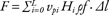
where v_p is gate-perpendicular, or perimeter-perpendicular, ice-surface velocity, H is the ice thickness, ρ is bulk ice-sheet density (assumed to be 915 ± 2 kg/m³) and f is the ratio of surface-to-depth-averaged ice velocity (assumed to be 0.93 ± 0.05; Thomas et al. 2001). Ice flux is summed along the PROMICE perimeter length (L) within a given ice-sheet sub-sector in increments (Δl) of 30 m. Gate-perpendicular velocity is calculated as:

where v is the absolute surface velocity and ϑ is the difference between ice flow and gate-perpendicular azimuths. When ϑ exceeds 90°, gate-perpendicular velocity becomes negative, indicating ice flow into the perimeter (Fig. 3). This reverse ice inflow occurs along 5.1% of the entire PROMICE perimeter (275 km), primarily in East Greenland.

Fig. 3.  A: Satellite-derived annual winter ice-velocity data availability along the PROMICE perimeter within the combined Joughin et al. (2010) and Rignot & Mouginot (2012) datasets during winters 1995–2015. B: 2008/2009 ice flow and gate-perpendicular azimuths around the PROMICE perimeter (Rignot & Mouginot 2012). C: Dimensionless scale factor (cos ϑ) of velocity magnitude. D: Absolute and gate-perpendicular surface velocity around the PROMICE perimeter. E: Changes in gate-perpendicular ice velocities surveyed in 2008/2009 and 2014/2015 (Joughin et al. 2010). In all subplots vertical dashed lines denote major glaciers (Fig. 1).

Grounding-line ice discharge (D) is calculated as the sum of ice flux across the PROMICE perimeter (F) and two downstream corrections that account for changing ice volume and surface mass balance:

where V̇_ds is the area-integrated observed rate of change in ice volume downstream of the perimeter, and ḃ_ds is the area-integrated modelled surface mass balance downstream of the perimeter. The rate of change in downstream ice volume captures changes due to both surface mass balance and ice dynamics. This requires the secondary surface mass balance correction to isolate the ice dynamic contribution to grounding-line ice discharge. Subtracting a negative downstream volume change increases ice flux, while adding a negative downstream surface mass balance decreases ice flux.

We assess mass balance (ṁ) within a given ice-sheet sub-sector as:

where ṁ is area-integrated modelled surface mass balance and D is calculated grounding-line ice discharge. We assess mass balance in eighteen of nineteen ice-sheet sub-sectors delineated by Zwally et al. (2012) using the PROMICE ice-sheet mask (Citterio & Ahlstrøm 2013). These eighteen minor sub-sectors are aggregated into eight major sectors (Fig. 1A). We do not assess mass balance in Sector 3.2 (Geikie Plateau). We propagate the uncertainties following Andersen et al. (2015), whereby we employ quadratic sums for terms with common units and quadratic fractional sums for terms with differing units.

Datasets

We interpolate satellite-derived synthetic aperture radar ice velocity (v) along the PROMICE perimeter from a spatially complete and temporally constrained winter 2008/2009 velocity mosaic of 150 m spatial resolution (Rignot & Mouginot 2012). Where possible – along 67% of the PROMICE perimeter – we derive temporal trends in ice velocity from overlapping winter 2008/2009 and winter 2014/2015 velocity mosaics (Joughin et al. 2010). We apply these temporal trends within each sub-sector to estimate annual perimeter velocity profiles during the 2000–2015 period. This approach is meant to complement the spatial completeness of the Rignot & Mouginot (2012) annual mosaic with the temporal repeat of the Joughin et al. (2010) data. We assume the perimeter velocity profile in the year 2000 is characteristic of the 1995–1999 period, on the basis that the ice-sheet interior was near equilibrium mass balance prior to 2000 (Thomas et al. 2001). These simplifications overlook pre-2008 ice flow variability, such as the acceleration and deceleration of South-East Greenland glaciers during 2000–2007 (Enderlin et al. 2014). While pre-2008 ice-sheet velocity maps are available, their quality decreases inland from the ice-sheet margin, which results in poor sampling along the PROMICE perimeter (Fig. 3).

We estimate ice thickness (H) along the PROMICE perimeter using ice surface and bed elevation data. Where possible, ice thickness is calculated from PROMICE airborne campaign laser and radar altimetry measurements in 2007, 2011 and 2015 (Sørensen et al. 2018). PROMICE airborne radar surveys have measured bedrock elevation along 79% of the perimeter. Bedrock elevations are interpolated along the remaining 21% of the perimeter from BedMachine v3 (Morlighem et al. 2017). PROMICE laser altimetry surveys each measured ice-sheet surface elevation along 74 to 79% of the perimeter. Along 15% of the perimeter never surveyed by airborne altimetry, ice-sheet surface elevations are interpolated from a digital elevation model representative of 2007 (Howat et al. 2014). When and where required, independent altimetry-derived rates of elevation change are used to derive annual elevation profiles along the perimeter during 2000–2015 (Khan et al. 2016).

We interpolate area-integrated rate of change in ice volume observed downstream of the PROMICE perimeter (V̇_ds) annually within each ice-sheet sub-sector during the 1995–2015 period from the same independent air- and satellite-borne altimetry product (Khan et al. 2016). These rates of volume change have been corrected for firn compaction when and where necessary. We estimate rates of change in ice volume in each sub-sector by area-integrating this altimetry product, and associated uncertainties, at 500 m spatial resolution, over the ice-sheet area downstream of the PROMICE perimeter (Citterio & Ahlstrøm 2013).

We use surface mass balance simulated by the MAR3.5.2 regional climate model for both downstream surface mass balance correction (ḃ_ds) and assessing ice-sheet wide surface mass balance input (ḃ). This permits us to assimilate the runoff and snowfall rates of a four-simulation ensemble reflecting four different climate forcings (ERA-20C, ERA-Interim, NCEPv1 and 20CRv2c) into an annual surface mass balance time series that spans 1980–2015 at 500 m spatial resolution. We remove relative anomalies between these four simulations during the common 1980–1999 period (Fettweis et al. 2017). The PROMICE ice-sheet mask we employ has a more extensive ice-sheet ablation area than the native MAR3.5.2 ice mask (Citterio & Ahlstrøm 2013). Relative to the native 25 km MAR ice mask, the more extensive ice-sheet ablation area of the 500 m PROMICE ice mask decreases ice-sheet integrated surface mass balance by c. 30 Gt/yr. The ice-sheet integrated downscaled surface mass balance we interpolate is within the range of independently elevation-dependent downscaled MAR2 simulations (Franco et al. 2012).

Ice sheet mass loss

Our updated input-output assessment gives a total 1995– 2015 ice-sheet mass loss of 3028 ± 711 Gt (Fig. 4). This is equivalent to a eustatic sea-level rise contribution of 8.4 ± 1.9 mm. We assess all eight major ice-sheet sectors as within uncertainty of equilibrium balance at the start of the survey period (c. 1995). Negative mass balance years, however, have clearly become more common towards the end of the survey period (Fig. 4). In particular, marine-terminating sectors with substantial ice discharge (central West (7), South-East (4) and North-East (8)) transitioned to persistent mass loss c. 2002, 2004 and 2005, respectively. Land-terminating sectors with substantial meltwater runoff (South (5), South-West (6)) subsequently transitioned to persistent mass loss c. 2006.

Fig. 4.  Annual surface mass balance, ice discharge and mass balance in eight major ice-sheet sectors (1–8), as well as for the entire ice sheet, over the 1995– 2015 period. Vertical spread denotes associated uncertainty. Map: Spatial distribution of the average 1995–2015 mass balance (MB) within the PROMICE ice-sheet mask (Citterio & Ahlstrøm 2013; Khan et al. 2016). Black lines denote the eight major ice-sheet sectors (Zwally et al. 2012).

At the ice-sheet scale, the total mass loss we assess over the 1995–2011 period agrees, within uncertainty, with that assessed by the Ice Sheet Mass Balance Inter-Comparison Exercise (IMBIE) (Fig. 5; Shepherd et al. 2012). The apparent discrepancy between IMBIE and PROMICE mass loss estimates is approximately equivalent to independent estimates of peripheral glacier mass loss (Noël et al. 2017). Adding the PROMICE mass loss estimate for the ice sheet proper with the peripheral glacier mass loss estimate of Noël et al. (2017) suggests that peripheral glaciers were responsible for 17 ± 7% of Greenland’s contribution to sea level change during 2004–2013. Peripheral glaciers account for < 5% of Greenland’s ice-covered area (Citterio & Ahlstrøm, 2013), making their specific, or per unit area, sea-level contribution disproportionately greater than the ice sheet. Our linear extrapolation of pre-2008 ice velocities, under-sampling flow variations in South-East Greenland glaciers in 2000–2007, likely contributes to some discrepancy with the IMBIE sea-level contribution curve (Enderlin et al. 2014).

Fig. 5.  Cumulative sea-level equivalent (SLE) contribution from this PROMICE study shown in comparison to the Greenland Mass Balance Inter-Comparison Exercise (IMBIE; Shepherd et al. 2012). As IMBIE surveys both the ice sheet and peripheral glaciers, we also sum this study with the independent peripheral glacier contribution estimate of Noël et al. (2017) for context.

Ice discharge increased from 1995 (350 ± 72 Gt/yr) to 2009 (487 ± 71 Gt/yr), before decreasing slightly to 2015 (465 ± 74 Gt/yr). Persistently increasing trends in iceberg calving are more readily apparent in Sectors 7 and 8 than in Sectors 3 (Central East) and 4 (Fig. 4). The trend in ice flux across the PROMICE perimeter ( 1.5 Gt/yr/yr) was small in comparison to the trend in ice discharge across the grounding line ( 7.2 Gt/yr/yr) during 2000–2015. The majority of the inter-annual variability in grounding-line ice discharge therefore results from the downstream surface mass balance and ice volume corrections we apply to the perimeter flux. Ice-sheet wide ice discharge during 2000–2015 (432 ± 74 Gt/yr) is c. 45 Gt/yr (10%) lower than that assessed by King et al. (2018) (479 ± 20 Gt/yr) for the same period. During 2000–2010, our ice discharge (422 ± 74 Gt/yr) is c. 90 Gt/yr (21%) lower than that assessed by Enderlin et al. (2014; 511 ± 30 Gt/yr) during the same period. The formal uncertainty of a given study can therefore be substantially smaller than inter-study discrepancies.

Trends and variability in MAR-simulated ice-sheet wide surface mass balance have been widely discussed (Fettweis et al. 2017). The ice-sheet wide annual surface mass balances we employ are consistent with the relatively extensive ablation area of the 500 m resolution PROMICE ice mask and the average surface mass balance we interpolate over the 1990–2010 period (382 ± 58 Gt/yr) is within the sensitivity range of the elevation-dependent downscaled product of MAR2 simulations from their native 25 km resolution to 15 km resolution during the same period (Franco et al. 2012). As virtually the entire ice-sheet ablation area is downstream of the PROMICE perimeter, the ice discharge we assess is fundamentally dependent on simulated surface mass balance. A more positive surface mass balance simulation would result in greater ice discharge and vice versa. Differences in downstream surface mass balance correction are primarily responsible for the c. 55 Gt/yr (12%) decrease in the ice discharge assessed here (460 ± 75 Gt/yr) in comparison to that originally assessed by Andersen et al. (2015; 515 ± 57 Gt/yr) during 2007 and 2011.

Programme outlook

This report updates the contribution of the Greenland ice sheet to annual sea-level rise assessed by PROMICE, using the Andersen et al. (2015) input-output approach. We assess an ice-sheet mass loss of 3028 ± 711 Gt over the 1995–2015 period, which is equivalent to a eustatic sea-level rise contribution of 8.4 ± 1.9 mm. Combining our estimate of ice-sheet mass loss with a previous estimate of peripheral glacier mass loss yields a total Greenland ice loss (ice sheet plus peripheral glaciers) that is consistent with the most recent consensus of total Greenland ice loss (Shepherd et al. 2012; Noël et al. 2017). Digital versions of the area-integrated calendar year mass balance that we assess in eighteen ice-sheet sub-sectors, as well as underlying components, are available on the www.promice.dk website.

As a result of the relatively high-elevation and inland location of the PROMICE perimeter, virtually the entire ice-sheet ablation area resides downstream. This makes inter-annual variability in grounding-line ice discharge estimated by Andersen et al. (2015), highly sensitive to inter-annual variability in downstream corrections. Future PROMICE mass balance products will therefore adopt new approaches where ice flux is estimated across gates near the grounding lines of individual outlet glaciers. The sustained effort of the Programme for Monitoring of the Greenland Ice Sheet (PROMICE) will continue to provide Danish and international stakeholders open access to policy-relevant estimates of ice-sheet mass loss and sea-level rise.

Acknowledgements

This work is a product of the Programme for Monitoring of the Greenland Ice Sheet (www.PROMICE.dk), which is funded by the Danish Cooperation for Environment in the Arctic (DANCEA) through the Danish Ministry of Climate, Energy and Utilities. We thank the reviewers, Rachel Carr and Ellyn Enderlin, for their comments, which improved the manuscript.

References

Andersen et al. 2015: Basin-scale partitioning of Greenland ice sheet mass balance components (2007–2011). Earth and Planetary Science Letters 409, 89–95. https://dx.doi.org/10.1016/j.epsl.2014.10.015

Citterio, M. & Ahlstrøm, A. 2013: The aerophotogrammetric map of Greenland ice masses. The Cryosphere 7, 445–449. https://dx.doi.org/10.5194/tcd-6-3891-2012

Enderlin, E.M., Howat, I.M., Jeong, S., Noh, M.J., van Angelen, J.H., & van den Broeke, M.R. 2014. An improved mass budget for the Greenland ice sheet. Geophysical Research Letters 41, 866–972. https://dx.doi.org/10.1002/2013gl059010

Fettweis et al. 2017: Reconstructions of the 1900–2015 Greenland ice sheet surface mass balance using the regional climate MAR model. The Cryosphere 11, 1015–1033. https://dx.doi.org/10.5194/tc-11-1015-2017

Franco, B., Fettweis, X., Lang, C., & Erpicum, M. 2012: Impact of spatial resolution on the modelling of the Greenland ice sheet surface mass balance between 1990–2010 using the regional climate model MAR. The Cryosphere 6, 695–711. https://dx.doi.org/10.5194/tcd-6-635-2012

Howat, I.M., Negrete, A. & Smith, B.E. 2014: The Greenland Ice Mapping Project (GIMP) land classification and surface elevation data sets. The Cryosphere 8, 1509–1518. https://dx.doi.org/10.5194/tc-8-1509-2014

Joughin, I., Smith, B.E., Howat, I.M., Scambos, T., & Moon, T. 2010: Greenland flow variability from ice-sheet-wide velocity mapping. Journal of Glaciology 56, 415–430. https://dx.doi.org/10.3189/002214310792447734

King, M.D., Howat, I.M., Jeong, S., Noh, M.J., Wouters, B., Noël, B., & van den Broeke, M.R. 2018: Seasonal to decadal variability in ice discharge from the Greenland Ice Sheet. The Cryosphere 12, 3813–3825. https://doi.org/10.5194/tc-12-3813-2018

Khan et al. 2016: Geodetic measurements reveal similarities between post–Last Glacial Maximum and present-day mass loss from the Greenland ice sheet. Science Advances 2, e1600931. https://dx.doi.org/10.1126/sciadv.1600931

Morlighem et al. 2017: BedMachine v3: Complete Bed Topography and Ocean Bathymetry Mapping of Greenland From Multibeam Echo Sounding Combined With Mass Conservation. Geophysical Research Letters 44, 11,051–11,061. https://dx.doi.org/10.1002/2017gl074954

Noël et al. 2017: A tipping point in refreezing accelerates mass loss of Greenland’s glaciers and ice caps. Nature Communications 8, 14730. https://doi.org/10.1038/ncomms14730

Rignot, E. & M. Mouginot 2012: Ice flow in Greenland for the International Polar Year 2008–2009. Geophysical Research Letters 39, L11501. https://doi.org/10.1029/2012gl051634

Shepherd et al. 2012: A Reconciled Estimate of Ice-Sheet Mass Balance. Science 338, 1183–1190. https://doi.org/10.1126/science.1228102

Sørensen, L., Simonsen, S., Forsberg, R., Stenseng, L., Skourup, H., Kristensen S., & Colgan, W. 2018: Circum-Greenland ice thickness measurements collected during airborne PROMICE surveys in 2007, 2011 and 2015. Bulletin of the Geological Survey of Denmark and Greenland, 41, 79–82.

Thomas, R., Csatho, B., Davis, C., Kim, C., Krabill, W., Manizade, S., McConnell, J., & Sonntag, J. 2001: Mass balance of higher-elevation parts of the Greenland ice sheet. Journal of Geophysical Research 106, 33,707–33,716. https://doi.org/10.1029/2001jd900033

Zwally, H., Giovinetto, M., Beckley, M., & Saba, J. 2012: Antarctic and Greenland Drainage Systems. Digital Media. http://icesat4.gsfc.nasa.gov/cryo_data/ant_grn_drainage_systems.php

How to cite

Colgan, W., Mankoff, K.D., Kjeldsen, K.K., Bjørk, A.A., Box, J.E., Simonsen, S.B., Sørensen, L.S., Khan, S.A., Solgaard, A.M., Forsberg, R., Skourup, H., Stenseng, L., Kristensen, L.S., Hvidegaard, S.M., Citterio, M., Karlsson, N., Fettweis, X., Ahlstrøm, A.P., Andersen, S.B., van As, D., Fausto1, R.S. 2019: Greenland ice sheet mass balance assessed by PROMICE (1995–2015). Geological Survey of Denmark and Greenland Bulletin 43, e2019430201. https://doi.org/10.34194/GEUSB-201943-02-01